Probabilistic Forecasting: Bootstrapped Residuals¶

Forecasting intervals with bootstrapped residuals is a method used to estimate the uncertainty in predictions by resampling past prediction errors (residuals). The goal is to generate prediction intervals that capture the variability in the forecast, giving a range of possible future values instead of just a single point estimate.

The error of a one-step-ahead forecast is defined as the difference between the actual value and the predicted value ($e_t=y_t-{\hat{y}}_{t|t-1}$). By assuming that future errors will be similar to past errors, it is possible to simulate different predictions by taking samples from the collection of errors previously seen in the past (i.e., the residuals) and adding them to the predictions.

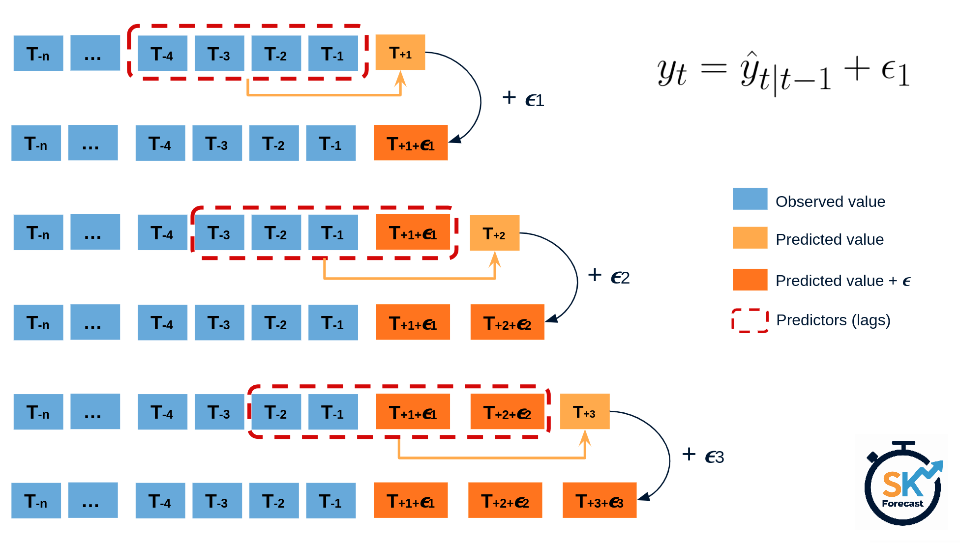
Diagram bootstrapping prediction process.

Repeatedly performing this process creates a collection of slightly different predictions, which represent the distribution of possible outcomes due to the expected variance in the forecasting process.

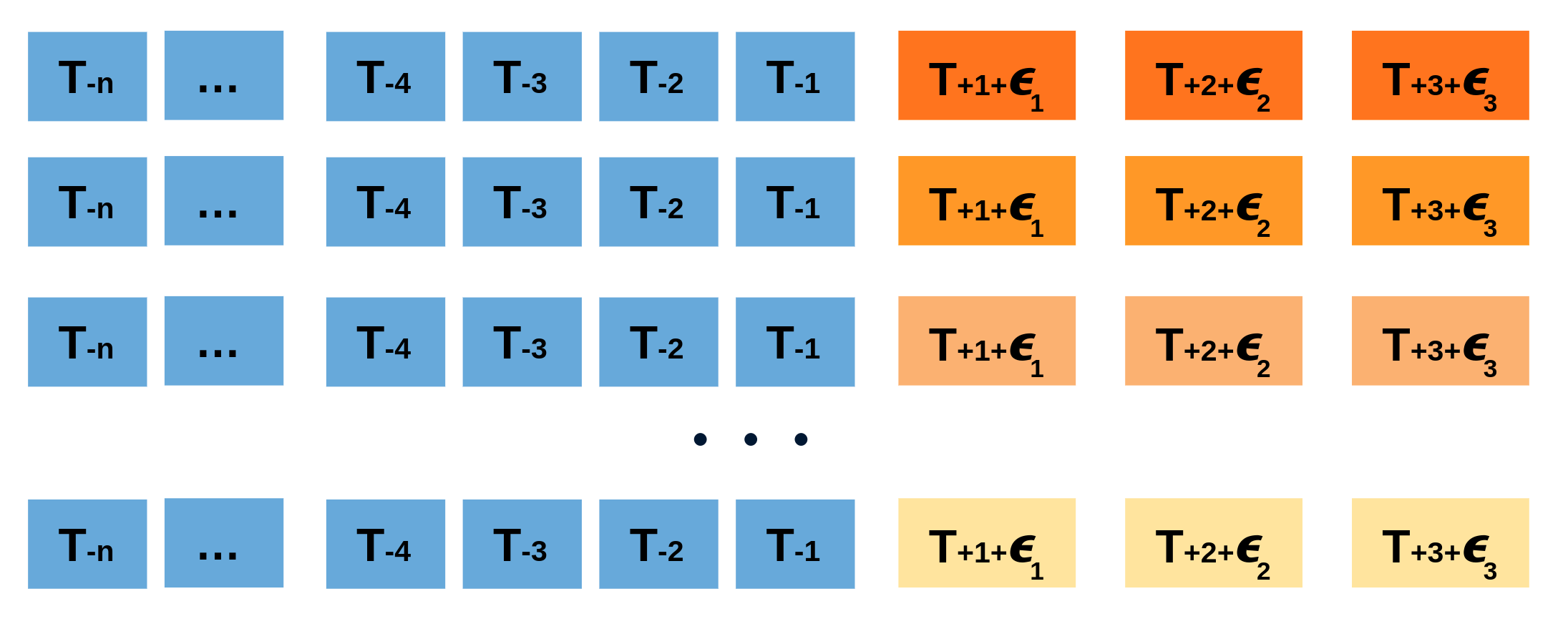
Bootstrapping predictions.

Using the outcome of the bootstrapping process, prediction intervals can be computed by calculating the $\alpha /2$ and $1-\alpha /2$ percentiles at each forecasting horizon.

Alternatively, it is also possible to fit a parametric distribution for each forecast horizon.

One of the main advantages of this strategy is that it requires only a single model to estimate any interval. However, performing hundreds or thousands of bootstrapping iterations can be computationally expensive and may not always be feasible.

💡 Tip

For more examples on how to use probabilistic forecasting, check out the following articles:

• Probabilistic forecasting with machine learning
• Probabilistic forecasting: prediction intervals for multi-step time series forecasting
• Continuous Ranked Probability Score (CRPS) in probabilistic forecasting

Libraries and data¶

In [1]:

# Data processing
# ==============================================================================
import numpy as np
import pandas as pd
from skforecast.datasets import fetch_dataset

# Plots
# ==============================================================================
import matplotlib.pyplot as plt
from skforecast.plot import (
    set_dark_theme,
    plot_residuals,
    plot_prediction_distribution,
    plot_prediction_intervals
)
from pprint import pprint

# Modelling and Forecasting
# ==============================================================================
from lightgbm import LGBMRegressor
from sklearn.pipeline import make_pipeline
from feature_engine.datetime import DatetimeFeatures
from feature_engine.creation import CyclicalFeatures
from skforecast.recursive import ForecasterRecursive
from skforecast.preprocessing import RollingFeatures
from skforecast.model_selection import TimeSeriesFold, backtesting_forecaster
from skforecast.metrics import calculate_coverage
from scipy.stats import norm

# Configuration
# ==============================================================================
import warnings
warnings.filterwarnings('once')

# Data processing # ============================================================================== import numpy as np import pandas as pd from skforecast.datasets import fetch_dataset # Plots # ============================================================================== import matplotlib.pyplot as plt from skforecast.plot import ( set_dark_theme, plot_residuals, plot_prediction_distribution, plot_prediction_intervals ) from pprint import pprint # Modelling and Forecasting # ============================================================================== from lightgbm import LGBMRegressor from sklearn.pipeline import make_pipeline from feature_engine.datetime import DatetimeFeatures from feature_engine.creation import CyclicalFeatures from skforecast.recursive import ForecasterRecursive from skforecast.preprocessing import RollingFeatures from skforecast.model_selection import TimeSeriesFold, backtesting_forecaster from skforecast.metrics import calculate_coverage from scipy.stats import norm # Configuration # ============================================================================== import warnings warnings.filterwarnings('once')

In [2]:

# Data download
# ==============================================================================
data = fetch_dataset(name='bike_sharing', raw=False)
data = data[['users', 'temp', 'hum', 'windspeed', 'holiday']]
data = data.loc['2011-04-01 00:00:00':'2012-10-20 23:00:00', :].copy()
data.head(3)

# Data download # ============================================================================== data = fetch_dataset(name='bike_sharing', raw=False) data = data[['users', 'temp', 'hum', 'windspeed', 'holiday']] data = data.loc['2011-04-01 00:00:00':'2012-10-20 23:00:00', :].copy() data.head(3)

bike_sharing
------------
Hourly usage of the bike share system in the city of Washington D.C. during the
years 2011 and 2012. In addition to the number of users per hour, information
about weather conditions and holidays is available.
Fanaee-T,Hadi. (2013). Bike Sharing Dataset. UCI Machine Learning Repository.
https://doi.org/10.24432/C5W894.
Shape of the dataset: (17544, 11)

Out[2]:

	users	temp	hum	windspeed	holiday
date_time
2011-04-01 00:00:00	6.0	10.66	100.0	11.0014	0.0
2011-04-01 01:00:00	4.0	10.66	100.0	11.0014	0.0
2011-04-01 02:00:00	7.0	10.66	93.0	12.9980	0.0

In [3]:

# Calendar features
# ==============================================================================
features_to_extract = [
    'month',
    'week',
    'day_of_week',
    'hour'
]
calendar_transformer = DatetimeFeatures(
    variables           = 'index',
    features_to_extract = features_to_extract,
    drop_original       = False,
)

# Cyclical encoding of calendar features
# ==============================================================================
features_to_encode = [
    "month",
    "week",
    "day_of_week",
    "hour",
]
max_values = {
    "month": 12,
    "week": 52,
    "day_of_week": 7,
    "hour": 24,
}
cyclical_encoder = CyclicalFeatures(
                       variables     = features_to_encode,
                       max_values    = max_values,
                       drop_original = True
                   )

exog_transformer = make_pipeline(
                       calendar_transformer,
                       cyclical_encoder
                   )

data = exog_transformer.fit_transform(data)
exog_features = data.columns.difference(['users']).tolist()
data.head(3)

# Calendar features # ============================================================================== features_to_extract = [ 'month', 'week', 'day_of_week', 'hour' ] calendar_transformer = DatetimeFeatures( variables = 'index', features_to_extract = features_to_extract, drop_original = False, ) # Cyclical encoding of calendar features # ============================================================================== features_to_encode = [ "month", "week", "day_of_week", "hour", ] max_values = { "month": 12, "week": 52, "day_of_week": 7, "hour": 24, } cyclical_encoder = CyclicalFeatures( variables = features_to_encode, max_values = max_values, drop_original = True ) exog_transformer = make_pipeline( calendar_transformer, cyclical_encoder ) data = exog_transformer.fit_transform(data) exog_features = data.columns.difference(['users']).tolist() data.head(3)

Out[3]:

	users	temp	hum	windspeed	holiday	month_sin	month_cos	week_sin	week_cos	day_of_week_sin	day_of_week_cos	hour_sin	hour_cos
date_time
2011-04-01 00:00:00	6.0	10.66	100.0	11.0014	0.0	0.866025	-0.5	1.0	6.123234e-17	-0.433884	-0.900969	0.000000	1.000000
2011-04-01 01:00:00	4.0	10.66	100.0	11.0014	0.0	0.866025	-0.5	1.0	6.123234e-17	-0.433884	-0.900969	0.258819	0.965926
2011-04-01 02:00:00	7.0	10.66	93.0	12.9980	0.0	0.866025	-0.5	1.0	6.123234e-17	-0.433884	-0.900969	0.500000	0.866025

In [4]:

# Split train-validation-test
# ==============================================================================
end_train = '2012-06-30 23:59:00'
end_validation = '2012-10-01 23:59:00'
data_train = data.loc[: end_train, :]
data_val   = data.loc[end_train:end_validation, :]
data_test  = data.loc[end_validation:, :]

print(f"Dates train      : {data_train.index.min()} --- {data_train.index.max()}  (n={len(data_train)})")
print(f"Dates validation : {data_val.index.min()} --- {data_val.index.max()}  (n={len(data_val)})")
print(f"Dates test       : {data_test.index.min()} --- {data_test.index.max()}  (n={len(data_test)})")

# Split train-validation-test # ============================================================================== end_train = '2012-06-30 23:59:00' end_validation = '2012-10-01 23:59:00' data_train = data.loc[: end_train, :] data_val = data.loc[end_train:end_validation, :] data_test = data.loc[end_validation:, :] print(f"Dates train : {data_train.index.min()} --- {data_train.index.max()} (n={len(data_train)})") print(f"Dates validation : {data_val.index.min()} --- {data_val.index.max()} (n={len(data_val)})") print(f"Dates test : {data_test.index.min()} --- {data_test.index.max()} (n={len(data_test)})")

Dates train      : 2011-04-01 00:00:00 --- 2012-06-30 23:00:00  (n=10968)
Dates validation : 2012-07-01 00:00:00 --- 2012-10-01 23:00:00  (n=2232)
Dates test       : 2012-10-02 00:00:00 --- 2012-10-20 23:00:00  (n=456)

In [5]:

# Plot partitions
# ==============================================================================
set_dark_theme()
plt.rcParams['lines.linewidth'] = 0.5
fig, ax = plt.subplots(figsize=(8, 3))
ax.plot(data_train['users'], label='Train')
ax.plot(data_val['users'], label='Validation')
ax.plot(data_test['users'], label='Test')
ax.set_title('users')
ax.legend();

# Plot partitions # ============================================================================== set_dark_theme() plt.rcParams['lines.linewidth'] = 0.5 fig, ax = plt.subplots(figsize=(8, 3)) ax.plot(data_train['users'], label='Train') ax.plot(data_val['users'], label='Validation') ax.plot(data_test['users'], label='Test') ax.set_title('users') ax.legend();

Intervals with In-sample residuals¶

By default, intervals can be computed using in-sample residuals (residuals from the training set), either by calling the predict_interval() method, or by performing a full backtesting procedure. However, this can result in intervals that are too narrow (overly optimistic).

✎ Note

Hiperparametrs used in this example have been previusly optimized using a bayesian search process. For more information about this process, please refer to: Hyperparameter tuning and lags selection.

In [6]:

# Create and fit forecaster
# ==============================================================================
params = {
    "max_depth": 7,
    "n_estimators": 300,
    "learning_rate": 0.06,
    "verbose": -1,
    "random_state": 15926
}
lags = [1, 2, 3, 23, 24, 25, 167, 168, 169]
window_features = RollingFeatures(stats=["mean"], window_sizes=24 * 3)

forecaster = ForecasterRecursive(
                 regressor       = LGBMRegressor(**params),
                 lags            = lags,
                 window_features = window_features,
             )

forecaster.fit(
    y    = data.loc[:end_validation, 'users'],
    exog = data.loc[:end_validation, exog_features],
    store_in_sample_residuals = False
)

# Create and fit forecaster # ============================================================================== params = { "max_depth": 7, "n_estimators": 300, "learning_rate": 0.06, "verbose": -1, "random_state": 15926 } lags = [1, 2, 3, 23, 24, 25, 167, 168, 169] window_features = RollingFeatures(stats=["mean"], window_sizes=24 * 3) forecaster = ForecasterRecursive( regressor = LGBMRegressor(**params), lags = lags, window_features = window_features, ) forecaster.fit( y = data.loc[:end_validation, 'users'], exog = data.loc[:end_validation, exog_features], store_in_sample_residuals = False )

By default, store_in_sample_residuals is set to False to speed up the training process. To store in-sample residuals without retraining the model, you can call the set_in_sample_residuals() method and pass the training data or set store_in_sample_residuals to True when fitting the model.

In [7]:

# Store in-sample residuals in case store_in_sample_residuals = False
# ==============================================================================
forecaster.set_in_sample_residuals(
    y    = data.loc[:end_validation, 'users'],
    exog = data.loc[:end_validation, exog_features]
)

# Store in-sample residuals in case store_in_sample_residuals = False # ============================================================================== forecaster.set_in_sample_residuals( y = data.loc[:end_validation, 'users'], exog = data.loc[:end_validation, exog_features] )

In [8]:

# In-sample residuals stored during fit
# ==============================================================================
print("Amount of residuals stored:", len(forecaster.in_sample_residuals_))
forecaster.in_sample_residuals_

# In-sample residuals stored during fit # ============================================================================== print("Amount of residuals stored:", len(forecaster.in_sample_residuals_)) forecaster.in_sample_residuals_

Amount of residuals stored: 10000

Out[8]:

array([ 42.02327339,  -4.75342728, -39.26777553, ...,  -3.54886809,
       -41.20842177, -13.42207696])

The backtesting_forecaster() function is used to estimate the prediction intervals for the entire test set. Few arguments are required to use this function:

• use_in_sample_residuals: If True, the in-sample residuals are used to compute the prediction intervals. Since these residuals are obtained from the training set, they are always available, but usually lead to overoptimistic intervals. If False, the out-sample residuals are used to calculate the prediction intervals. These residuals are obtained from the validation set and are only available if the set_out_sample_residuals() method has been called. It is recommended to use out-sample residuals to achieve the desired coverage.

• The interval argument indicates the quantiles used to calculate the prediction intervals. For example, if the 10th and 90th percentiles are used, the resulting prediction intervals will have a nominal coverage of 80%.

• interval_method is used to specify the method used to calculate the prediction intervals. In this case, the bootstrapped method is used but other methods are available.

• The n_boot argument is used to specify the number of bootstrap samples to be used in estimating the prediction intervals. The larger the number of samples, the more accurate the prediction intervals will be, but the longer the calculation will take.

In [9]:

# Backtesting with prediction intervals in test data using in-sample residuals
# ==============================================================================
cv = TimeSeriesFold(
         steps              = 24, 
         initial_train_size = len(data.loc[:end_validation]),
         refit              = False
     )

metric, predictions = backtesting_forecaster(
                          forecaster              = forecaster,
                          y                       = data['users'],
                          exog                    = data[exog_features],
                          cv                      = cv,
                          metric                  = 'mean_absolute_error',
                          interval                = [10, 90],  # 80% prediction interval
                          interval_method         = 'bootstrapping',
                          n_boot                  = 150,
                          use_in_sample_residuals = True,  # Use in-sample residuals
                          use_binned_residuals    = False
                      )
predictions.head(5)

# Backtesting with prediction intervals in test data using in-sample residuals # ============================================================================== cv = TimeSeriesFold( steps = 24, initial_train_size = len(data.loc[:end_validation]), refit = False ) metric, predictions = backtesting_forecaster( forecaster = forecaster, y = data['users'], exog = data[exog_features], cv = cv, metric = 'mean_absolute_error', interval = [10, 90], # 80% prediction interval interval_method = 'bootstrapping', n_boot = 150, use_in_sample_residuals = True, # Use in-sample residuals use_binned_residuals = False ) predictions.head(5)

  0%|          | 0/19 [00:00<?, ?it/s]

Out[9]:

	pred	lower_bound	upper_bound
2012-10-02 00:00:00	58.387527	32.799491	78.248425
2012-10-02 01:00:00	17.870302	-7.253084	50.190172
2012-10-02 02:00:00	7.901576	-17.057776	37.596425
2012-10-02 03:00:00	5.414332	-16.809510	40.194483
2012-10-02 04:00:00	10.379630	-12.696466	56.904041

In [10]:

# Plot intervals
# ==============================================================================
plot_prediction_intervals(
    predictions         = predictions,
    y_true              = data_test,
    target_variable     = "users",
    title               = "Prediction intervals in test data",
    kwargs_fill_between = {'color': 'gray', 'alpha': 0.3, 'zorder': 1}
)

# Predicted interval coverage (on test data)
# ==============================================================================
coverage = calculate_coverage(
               y_true      = data.loc[end_validation:, 'users'],
               lower_bound = predictions["lower_bound"], 
               upper_bound = predictions["upper_bound"]
           )
print(f"Predicted interval coverage: {round(100 * coverage, 2)} %")

# Area of the interval
# ==============================================================================
area = (predictions["upper_bound"] - predictions["lower_bound"]).sum()
print(f"Area of the interval: {round(area, 2)}")

# Plot intervals # ============================================================================== plot_prediction_intervals( predictions = predictions, y_true = data_test, target_variable = "users", title = "Prediction intervals in test data", kwargs_fill_between = {'color': 'gray', 'alpha': 0.3, 'zorder': 1} ) # Predicted interval coverage (on test data) # ============================================================================== coverage = calculate_coverage( y_true = data.loc[end_validation:, 'users'], lower_bound = predictions["lower_bound"], upper_bound = predictions["upper_bound"] ) print(f"Predicted interval coverage: {round(100 * coverage, 2)} %") # Area of the interval # ============================================================================== area = (predictions["upper_bound"] - predictions["lower_bound"]).sum() print(f"Area of the interval: {round(area, 2)}")

Predicted interval coverage: 61.84 %
Area of the interval: 43177.89

The prediction intervals show overconfidence as they tend to be too narrow, resulting in a true coverage well below the nominal coverage of 80%. This phenomenon is due to the tendency of the in-sample residuals to often overestimate the predictive ability of the model.

In [11]:

# Store results for later comparison
# ==============================================================================
predictions_in_sample_residuals = predictions.copy()

# Store results for later comparison # ============================================================================== predictions_in_sample_residuals = predictions.copy()

Out-sample residuals (non-conditioned on predicted values)¶

To address the issue of overoptimistic intervals, it is possible to use out-sample residuals (residuals from a validation set not seen during training) to estimate the prediction intervals. These residuals can be obtained through backtesting.

In [12]:

# Backtesting on validation data to obtain out-sample residuals
# ==============================================================================
cv = TimeSeriesFold(
         steps              = 24, 
         initial_train_size = len(data.loc[:end_train]),
         refit              = False
     )

_, predictions_val = backtesting_forecaster(
                         forecaster    = forecaster,
                         y             = data.loc[:end_validation, 'users'],
                         exog          = data.loc[:end_validation, exog_features],
                         cv            = cv,
                         metric        = 'mean_absolute_error'
                     )

# Backtesting on validation data to obtain out-sample residuals # ============================================================================== cv = TimeSeriesFold( steps = 24, initial_train_size = len(data.loc[:end_train]), refit = False ) _, predictions_val = backtesting_forecaster( forecaster = forecaster, y = data.loc[:end_validation, 'users'], exog = data.loc[:end_validation, exog_features], cv = cv, metric = 'mean_absolute_error' )

  0%|          | 0/93 [00:00<?, ?it/s]

In [13]:

# Out-sample residuals distribution
# ==============================================================================
residuals = data.loc[predictions_val.index, 'users'] - predictions_val['pred']
print(pd.Series(np.where(residuals < 0, 'negative', 'positive')).value_counts())
plt.rcParams.update({'font.size': 8})
_ = plot_residuals(residuals=residuals, figsize=(7, 4))

# Out-sample residuals distribution # ============================================================================== residuals = data.loc[predictions_val.index, 'users'] - predictions_val['pred'] print(pd.Series(np.where(residuals < 0, 'negative', 'positive')).value_counts()) plt.rcParams.update({'font.size': 8}) _ = plot_residuals(residuals=residuals, figsize=(7, 4))

positive    1297
negative     935
Name: count, dtype: int64

With the set_out_sample_residuals() method, the out-sample residuals are stored in the forecaster object so that they can be used to calibrate the prediction intervals.

In [14]:

# Store out-sample residuals in the forecaster
# ==============================================================================
forecaster.set_out_sample_residuals(
    y_true = data.loc[predictions_val.index, 'users'], 
    y_pred = predictions_val['pred']
)

# Store out-sample residuals in the forecaster # ============================================================================== forecaster.set_out_sample_residuals( y_true = data.loc[predictions_val.index, 'users'], y_pred = predictions_val['pred'] )

Now that the new residuals have been added to the forecaster, the prediction intervals can be calculated using use_in_sample_residuals = False.

In [15]:

# Backtesting with prediction intervals in test data using out-sample residuals
# ==============================================================================
cv = TimeSeriesFold(
         steps              = 24, 
         initial_train_size = len(data.loc[:end_validation]),
         refit              = False
     )

metric, predictions = backtesting_forecaster(
                          forecaster              = forecaster,
                          y                       = data['users'],
                          exog                    = data[exog_features],
                          cv                      = cv,
                          metric                  = 'mean_absolute_error',
                          interval                = [10, 90],  # 80% prediction interval
                          interval_method         = 'bootstrapping',
                          n_boot                  = 150,
                          use_in_sample_residuals = False,  # Use out-sample residuals
                          use_binned_residuals    = False
                      )
predictions.head(5)

# Backtesting with prediction intervals in test data using out-sample residuals # ============================================================================== cv = TimeSeriesFold( steps = 24, initial_train_size = len(data.loc[:end_validation]), refit = False ) metric, predictions = backtesting_forecaster( forecaster = forecaster, y = data['users'], exog = data[exog_features], cv = cv, metric = 'mean_absolute_error', interval = [10, 90], # 80% prediction interval interval_method = 'bootstrapping', n_boot = 150, use_in_sample_residuals = False, # Use out-sample residuals use_binned_residuals = False ) predictions.head(5)

  0%|          | 0/19 [00:00<?, ?it/s]

Out[15]:

	pred	lower_bound	upper_bound
2012-10-02 00:00:00	58.387527	30.961801	133.296285
2012-10-02 01:00:00	17.870302	-14.031592	132.635745
2012-10-02 02:00:00	7.901576	-32.265023	142.360525
2012-10-02 03:00:00	5.414332	-32.495340	167.312462
2012-10-02 04:00:00	10.379630	-13.725526	252.174056

In [16]:

# Plot intervals
# ==============================================================================
plot_prediction_intervals(
    predictions         = predictions,
    y_true              = data_test,
    target_variable     = "users",
    title               = "Prediction intervals in test data",
    kwargs_fill_between = {'color': 'gray', 'alpha': 0.3, 'zorder': 1}
)

# Predicted interval coverage (on test data)
# ==============================================================================
coverage = calculate_coverage(
               y_true      = data.loc[end_validation:, 'users'],
               lower_bound = predictions["lower_bound"], 
               upper_bound = predictions["upper_bound"]
           )
print(f"Predicted interval coverage: {round(100 * coverage, 2)} %")

# Area of the interval
# ==============================================================================
area = (predictions["upper_bound"] - predictions["lower_bound"]).sum()
print(f"Area of the interval: {round(area, 2)}")

# Plot intervals # ============================================================================== plot_prediction_intervals( predictions = predictions, y_true = data_test, target_variable = "users", title = "Prediction intervals in test data", kwargs_fill_between = {'color': 'gray', 'alpha': 0.3, 'zorder': 1} ) # Predicted interval coverage (on test data) # ============================================================================== coverage = calculate_coverage( y_true = data.loc[end_validation:, 'users'], lower_bound = predictions["lower_bound"], upper_bound = predictions["upper_bound"] ) print(f"Predicted interval coverage: {round(100 * coverage, 2)} %") # Area of the interval # ============================================================================== area = (predictions["upper_bound"] - predictions["lower_bound"]).sum() print(f"Area of the interval: {round(area, 2)}")

Predicted interval coverage: 83.33 %
Area of the interval: 101257.22

The resulting prediction intervals derived from the out-sample residuals are wider than those generated using the in-sample residuals. This results in an empirical coverage that is closer to the nominal coverage of 80%.

By zooming in on the plot, the reader will notice that the intervals are particularly wide when the predicted values are low, indicating that the model is not able to properly localize the uncertainty of its predictions.

In [17]:

# Plot intervals zoomed in ["2012-10-08 00:00:00", "2012-10-15 00:00:00"]
# ==============================================================================
plot_prediction_intervals(
    predictions     = predictions,
    y_true          = data_test,
    initial_x_zoom  = ["2012-10-08 00:00:00", "2012-10-15 00:00:00"],
    target_variable = "users",
    title           = "Prediction intervals in test data",
    kwargs_fill_between = {'color': 'gray', 'alpha': 0.3, 'zorder': 1}
)

# Plot intervals zoomed in ["2012-10-08 00:00:00", "2012-10-15 00:00:00"] # ============================================================================== plot_prediction_intervals( predictions = predictions, y_true = data_test, initial_x_zoom = ["2012-10-08 00:00:00", "2012-10-15 00:00:00"], target_variable = "users", title = "Prediction intervals in test data", kwargs_fill_between = {'color': 'gray', 'alpha': 0.3, 'zorder': 1} )

In [18]:

# Store results for later comparison
# ==============================================================================
predictions_out_sample_residuals = predictions.copy()

# Store results for later comparison # ============================================================================== predictions_out_sample_residuals = predictions.copy()

Intervals conditioned on predicted values (binned residuals)¶

The bootstrapping process assumes that the residuals are independently distributed so that they can be used independently of the predicted value. In reality, this is rarely true; in most cases, the magnitude of the residuals is correlated with the magnitude of the predicted value. In this case, for example, one would hardly expect the error to be the same when the predicted number of users is close to zero as when it is in the hundreds.

To account for the dependence between the residuals and the predicted values, skforecast allows to partition the residuals into K bins, where each bin is associated with a range of predicted values. Using this strategy, the bootstrapping process samples the residuals from different bins depending on the predicted value, which can improve the coverage of the interval while adjusting the width if necessary, allowing the model to better distribute the uncertainty of its predictions.

Internally, skforecast uses a QuantileBinner class to bin data into quantile-based bins using numpy.percentile. This class is similar to KBinsDiscretizer but faster for binning data into quantile-based bins. Bin intervals are defined following the convention: bins[i-1] <= x < bins[i]. The binning process can be adjusted using the argument binner_kwargs of the Forecaster object.

In [19]:

# Create and train forecaster
# ==============================================================================
forecaster = ForecasterRecursive(
                 regressor     = LGBMRegressor(**params),
                 lags          = lags,
                 binner_kwargs = {'n_bins': 10}   
             )

forecaster.fit(
    y    = data.loc[:end_validation, 'users'],
    exog = data.loc[:end_validation, exog_features],
    store_in_sample_residuals = True
)

# Create and train forecaster # ============================================================================== forecaster = ForecasterRecursive( regressor = LGBMRegressor(**params), lags = lags, binner_kwargs = {'n_bins': 10} ) forecaster.fit( y = data.loc[:end_validation, 'users'], exog = data.loc[:end_validation, exog_features], store_in_sample_residuals = True )

During the training process, the forecaster uses the in-sample predictions to define the intervals at which the residuals are stored depending on the predicted value to which they are related (binner_intervals_ attribute).

Although not used in this example, the in-sample residuals are divided into bins and stored in the in_sample_residuals_by_bin_ attribute.

In [20]:

# Intervals of the residual bins
# ==============================================================================
pprint(forecaster.binner_intervals_)

# Intervals of the residual bins # ============================================================================== pprint(forecaster.binner_intervals_)

{0: (-0.8943794883271247, 10.608406827878845),
 1: (10.608406827878845, 30.676160623625577),
 2: (30.676160623625577, 74.1882217425986),
 3: (74.1882217425986, 120.49652689276296),
 4: (120.49652689276296, 164.97690978552197),
 5: (164.97690978552197, 209.69596300954962),
 6: (209.69596300954962, 268.3808557231679),
 7: (268.3808557231679, 338.3331511270013),
 8: (338.3331511270013, 460.65535040899925),
 9: (460.65535040899925, 955.802117392104)}

In [21]:

# Number of in-sample residuals by bin
# ==============================================================================
for k, v in forecaster.in_sample_residuals_by_bin_.items():
    print(f"Bin {k}: n={len(v)}")

# Number of in-sample residuals by bin # ============================================================================== for k, v in forecaster.in_sample_residuals_by_bin_.items(): print(f"Bin {k}: n={len(v)}")

Bin 0: n=1000
Bin 1: n=1000
Bin 2: n=1000
Bin 3: n=1000
Bin 4: n=1000
Bin 5: n=1000
Bin 6: n=1000
Bin 7: n=1000
Bin 8: n=1000
Bin 9: n=1000

The set_out_sample_residuals() method will bin the residuals according to the intervals learned during fitting. To avoid using too much memory, the number of residuals stored per bin is limited to 10_000 // self.binner.n_bins_. The predictions obtained in the backtesting are used.

In [22]:

# Store out-sample residuals in the forecaster
# ==============================================================================
forecaster.set_out_sample_residuals(
    y_true = data.loc[predictions_val.index, 'users'], 
    y_pred = predictions_val['pred']
)

# Store out-sample residuals in the forecaster # ============================================================================== forecaster.set_out_sample_residuals( y_true = data.loc[predictions_val.index, 'users'], y_pred = predictions_val['pred'] )

In [23]:

# Number of out-sample residuals by bin
# ==============================================================================
for k, v in forecaster.out_sample_residuals_by_bin_.items():
    print(f"Bin {k}: n={len(v)}")

# Number of out-sample residuals by bin # ============================================================================== for k, v in forecaster.out_sample_residuals_by_bin_.items(): print(f"Bin {k}: n={len(v)}")

Bin 0: n=153
Bin 1: n=168
Bin 2: n=197
Bin 3: n=118
Bin 4: n=153
Bin 5: n=157
Bin 6: n=232
Bin 7: n=302
Bin 8: n=318
Bin 9: n=434

In [24]:

# Distribution of the residual by bin
# ==============================================================================
out_sample_residuals_by_bin_df = pd.DataFrame(
    dict(
        [(k, pd.Series(v))
         for k, v in forecaster.out_sample_residuals_by_bin_.items()]
    )
)
fig, ax = plt.subplots(figsize=(6, 3))
out_sample_residuals_by_bin_df.boxplot(
    flierprops=dict(marker='o', markerfacecolor='gray', markersize=6),
    ax=ax
)
ax.set_title("Distribution of residuals by bin", fontsize=12)
ax.set_xlabel("Bin", fontsize=10)
ax.set_ylabel("Residuals", fontsize=10)
plt.show();

# Distribution of the residual by bin # ============================================================================== out_sample_residuals_by_bin_df = pd.DataFrame( dict( [(k, pd.Series(v)) for k, v in forecaster.out_sample_residuals_by_bin_.items()] ) ) fig, ax = plt.subplots(figsize=(6, 3)) out_sample_residuals_by_bin_df.boxplot( flierprops=dict(marker='o', markerfacecolor='gray', markersize=6), ax=ax ) ax.set_title("Distribution of residuals by bin", fontsize=12) ax.set_xlabel("Bin", fontsize=10) ax.set_ylabel("Residuals", fontsize=10) plt.show();

The box plots show how the spread and magnitude of the residuals differ depending on the predicted value. The residuals are more dispersed when the predicted value is higher (higher bin), which is consistent with the intuition that errors tend to be larger when the predicted value is larger.

Finally, the prediction intervals estimated again, this time using out-sample residuals conditioned on the predicted values.

In [25]:

# Backtesting with prediction intervals in test data using out-sample residuals
# ==============================================================================
cv = TimeSeriesFold(
         steps              = 24, 
         initial_train_size = len(data.loc[:end_validation]),
         refit              = False
     )

metric, predictions = backtesting_forecaster(
                          forecaster              = forecaster,
                          y                       = data['users'],
                          exog                    = data[exog_features],
                          cv                      = cv,
                          metric                  = 'mean_absolute_error',
                          interval                = [10, 90],  # 80% prediction interval
                          interval_method         = 'bootstrapping',
                          n_boot                  = 150,
                          use_in_sample_residuals = False,  # Use out-sample residuals
                          use_binned_residuals    = True,   # Residuals conditioned on predicted values
                      )
predictions.head(3)

# Backtesting with prediction intervals in test data using out-sample residuals # ============================================================================== cv = TimeSeriesFold( steps = 24, initial_train_size = len(data.loc[:end_validation]), refit = False ) metric, predictions = backtesting_forecaster( forecaster = forecaster, y = data['users'], exog = data[exog_features], cv = cv, metric = 'mean_absolute_error', interval = [10, 90], # 80% prediction interval interval_method = 'bootstrapping', n_boot = 150, use_in_sample_residuals = False, # Use out-sample residuals use_binned_residuals = True, # Residuals conditioned on predicted values ) predictions.head(3)

  0%|          | 0/19 [00:00<?, ?it/s]

Out[25]:

	pred	lower_bound	upper_bound
2012-10-02 00:00:00	60.399647	40.609922	75.876519
2012-10-02 01:00:00	17.617464	5.186247	38.272262
2012-10-02 02:00:00	9.002365	4.862337	29.131771

In [26]:

# Plot intervals
# ==============================================================================
plot_prediction_intervals(
    predictions         = predictions,
    y_true              = data_test,
    target_variable     = "users",
    title               = "Prediction intervals in test data",
    xaxis_title         = "Date time",
    yaxis_title         = "users",
    kwargs_fill_between = {'color': 'gray', 'alpha': 0.3, 'zorder': 1}
)

# Predicted interval coverage (on test data)
# ==============================================================================
coverage = calculate_coverage(
               y_true      = data.loc[end_validation:, 'users'],
               lower_bound = predictions["lower_bound"], 
               upper_bound = predictions["upper_bound"]
           )
print(f"Predicted interval coverage: {round(100 * coverage, 2)} %")

# Area of the interval
# ==============================================================================
area = (predictions["upper_bound"] - predictions["lower_bound"]).sum()
print(f"Area of the interval: {round(area, 2)}")

# Plot intervals # ============================================================================== plot_prediction_intervals( predictions = predictions, y_true = data_test, target_variable = "users", title = "Prediction intervals in test data", xaxis_title = "Date time", yaxis_title = "users", kwargs_fill_between = {'color': 'gray', 'alpha': 0.3, 'zorder': 1} ) # Predicted interval coverage (on test data) # ============================================================================== coverage = calculate_coverage( y_true = data.loc[end_validation:, 'users'], lower_bound = predictions["lower_bound"], upper_bound = predictions["upper_bound"] ) print(f"Predicted interval coverage: {round(100 * coverage, 2)} %") # Area of the interval # ============================================================================== area = (predictions["upper_bound"] - predictions["lower_bound"]).sum() print(f"Area of the interval: {round(area, 2)}")

Predicted interval coverage: 85.96 %
Area of the interval: 96214.57

In [27]:

# Plot intervals zoomed in ["2012-10-08 00:00:00", "2012-10-15 00:00:00"]
# ==============================================================================
plot_prediction_intervals(
    predictions         = predictions,
    y_true              = data_test,
    initial_x_zoom      = ["2012-10-08 00:00:00", "2012-10-15 00:00:00"],
    target_variable     = "users",
    title               = "Prediction intervals in test data",
    kwargs_fill_between = {'color': 'gray', 'alpha': 0.3, 'zorder': 1}
)

# Plot intervals zoomed in ["2012-10-08 00:00:00", "2012-10-15 00:00:00"] # ============================================================================== plot_prediction_intervals( predictions = predictions, y_true = data_test, initial_x_zoom = ["2012-10-08 00:00:00", "2012-10-15 00:00:00"], target_variable = "users", title = "Prediction intervals in test data", kwargs_fill_between = {'color': 'gray', 'alpha': 0.3, 'zorder': 1} )

When using out-sample residuals conditioned on the predicted value, the area of the interval is significantly reduced and the uncertainty is mainly allocated to the predictions with high values. However, the empirical coverage is still above the expected coverage, which means that the estimated intervals are conservative.

The follwing plot compares the prediction intervals obtained using in-sample residuals, out-sample residuals, and out-sample residuals conditioned on the predicted values.

In [28]:

# Plot intervals using: in-sample residuals, out-sample residuals and binned residuals
# ==============================================================================
predictions_out_sample_residuals_binned = predictions.copy()
fig, ax = plt.subplots(figsize=(8, 4))
ax.fill_between(
    data_test.index,
    predictions_out_sample_residuals["lower_bound"],
    predictions_out_sample_residuals["upper_bound"],
    color='white',
    alpha=0.9,
    label='Out-sample residuals',
    zorder=1
)
ax.fill_between(
    data_test.index,
    predictions_out_sample_residuals_binned["lower_bound"],
    predictions_out_sample_residuals_binned["upper_bound"],
    color='#fc4f30',
    alpha=0.7,
    label='Out-sample binned residuals',
    zorder=2
)

ax.fill_between(
    data_test.index,
    predictions_in_sample_residuals["lower_bound"],
    predictions_in_sample_residuals["upper_bound"],
    color='#30a2da',
    alpha=0.9,
    label='In-sample residuals',
    zorder=3
)
ax.set_xlim(pd.to_datetime(["2012-10-08 00:00:00", "2012-10-15 00:00:00"]))
ax.set_title("Prediction intervals with different residuals", fontsize=12)
ax.legend();

# Plot intervals using: in-sample residuals, out-sample residuals and binned residuals # ============================================================================== predictions_out_sample_residuals_binned = predictions.copy() fig, ax = plt.subplots(figsize=(8, 4)) ax.fill_between( data_test.index, predictions_out_sample_residuals["lower_bound"], predictions_out_sample_residuals["upper_bound"], color='white', alpha=0.9, label='Out-sample residuals', zorder=1 ) ax.fill_between( data_test.index, predictions_out_sample_residuals_binned["lower_bound"], predictions_out_sample_residuals_binned["upper_bound"], color='#fc4f30', alpha=0.7, label='Out-sample binned residuals', zorder=2 ) ax.fill_between( data_test.index, predictions_in_sample_residuals["lower_bound"], predictions_in_sample_residuals["upper_bound"], color='#30a2da', alpha=0.9, label='In-sample residuals', zorder=3 ) ax.set_xlim(pd.to_datetime(["2012-10-08 00:00:00", "2012-10-15 00:00:00"])) ax.set_title("Prediction intervals with different residuals", fontsize=12) ax.legend();

⚠ Warning

Probabilistic forecasting in production

The correct estimation of prediction intervals with bootstrapped residuals depends on the residuals being representative of future errors. For this reason, out-of-sample residuals should be used. However, the dynamics of the series and models can change over time, so it is important to monitor and regularly update the residuals. It can be done easily using the set_out_sample_residuals() method.

Prediction of multiple intervals¶

The backtesting_forecaster function not only allows to estimate a single prediction interval, but also to estimate multiple quantiles (percentiles) from which multiple prediction intervals can be constructed. This is useful to evaluate the quality of the prediction intervals for a range of probabilities. Furthermore, it has almost no additional computational cost compared to estimating a single interval.

Next, several percentiles are predicted and from these, prediction intervals are created for different nominal coverage levels - 10%, 20%, 30%, 40%, 50%, 60%, 70%, 80%, 90% and 95% - and their actual coverage is assessed.

In [29]:

# Prediction intervals for different nominal coverages
# ==============================================================================
quantiles = [2.5, 5, 10, 15, 20, 25, 30, 35, 40, 45, 50, 55, 60, 65, 70, 75, 80, 85, 90, 95, 97.5]
intervals = [[2.5, 97.5], [5, 95], [10, 90], [15, 85], [20, 80], [30, 70], [35, 65], [40, 60], [45, 55]]
observed_coverages = []
observed_areas = []

metric, predictions = backtesting_forecaster(
                          forecaster              = forecaster,
                          y                       = data['users'],
                          exog                    = data[exog_features],
                          cv                      = cv,
                          metric                  = 'mean_absolute_error',
                          interval                = quantiles,
                          interval_method         = 'bootstrapping',
                          n_boot                  = 150,
                          use_in_sample_residuals = False,  # Use out-sample residuals
                          use_binned_residuals    = True
                      )
predictions.head()

# Prediction intervals for different nominal coverages # ============================================================================== quantiles = [2.5, 5, 10, 15, 20, 25, 30, 35, 40, 45, 50, 55, 60, 65, 70, 75, 80, 85, 90, 95, 97.5] intervals = [[2.5, 97.5], [5, 95], [10, 90], [15, 85], [20, 80], [30, 70], [35, 65], [40, 60], [45, 55]] observed_coverages = [] observed_areas = [] metric, predictions = backtesting_forecaster( forecaster = forecaster, y = data['users'], exog = data[exog_features], cv = cv, metric = 'mean_absolute_error', interval = quantiles, interval_method = 'bootstrapping', n_boot = 150, use_in_sample_residuals = False, # Use out-sample residuals use_binned_residuals = True ) predictions.head()

  0%|          | 0/19 [00:00<?, ?it/s]

Out[29]:

	pred	p_2.5	p_5	p_10	p_15	p_20	p_25	p_30	p_35	p_40	...	p_55	p_60	p_65	p_70	p_75	p_80	p_85	p_90	p_95	p_97.5
2012-10-02 00:00:00	60.399647	26.892402	33.951113	40.609922	42.760696	44.244359	46.570077	48.923822	49.785492	50.587951	...	55.370331	57.151158	58.458595	59.347441	61.621755	65.284405	69.355807	75.876519	86.239833	120.265754
2012-10-02 01:00:00	17.617464	2.689591	3.512207	5.186247	6.486508	8.169985	9.041067	9.761858	10.572733	11.359216	...	17.526959	19.567121	20.340357	23.363116	25.280020	29.001507	33.544834	38.272262	51.626343	71.371264
2012-10-02 02:00:00	9.002365	1.437432	2.099155	4.862337	5.415269	6.460628	6.985618	7.847532	8.239015	8.931894	...	11.559812	12.799507	13.812258	14.086847	15.113970	16.543545	20.604941	29.131771	35.799777	49.683165
2012-10-02 03:00:00	5.306644	-0.465970	1.157744	2.417394	3.083630	3.739066	4.018527	4.467039	5.003059	5.384454	...	6.667717	7.496738	8.055827	8.567819	9.560928	10.495075	12.231564	14.223768	19.437481	23.503909
2012-10-02 04:00:00	9.439573	-0.401817	2.997039	4.808793	5.552889	6.464636	6.875786	8.056258	8.496770	9.126208	...	10.863024	11.754925	12.132281	12.877582	13.524530	15.188979	18.552166	25.501337	30.655910	47.941695

5 rows × 22 columns

In [30]:

# Calculate coverage and area for each interval
# ==============================================================================
for interval in intervals:
    observed_coverage = calculate_coverage(
                            y_true      = data.loc[end_validation:, 'users'],
                            lower_bound = predictions[f"p_{interval[0]}"], 
                            upper_bound = predictions[f"p_{interval[1]}"]
                        )
    observed_area = (predictions[f"p_{interval[1]}"] - predictions[f"p_{interval[0]}"]).sum()
    observed_coverages.append(100 * observed_coverage)
    observed_areas.append(observed_area)

results = pd.DataFrame({
              'Interval': intervals,
              'Nominal coverage': [interval[1] - interval[0] for interval in intervals],
              'Observed coverage': observed_coverages,
              'Area': observed_areas
          })
results.round(1)

# Calculate coverage and area for each interval # ============================================================================== for interval in intervals: observed_coverage = calculate_coverage( y_true = data.loc[end_validation:, 'users'], lower_bound = predictions[f"p_{interval[0]}"], upper_bound = predictions[f"p_{interval[1]}"] ) observed_area = (predictions[f"p_{interval[1]}"] - predictions[f"p_{interval[0]}"]).sum() observed_coverages.append(100 * observed_coverage) observed_areas.append(observed_area) results = pd.DataFrame({ 'Interval': intervals, 'Nominal coverage': [interval[1] - interval[0] for interval in intervals], 'Observed coverage': observed_coverages, 'Area': observed_areas }) results.round(1)

Out[30]:

	Interval	Nominal coverage	Observed coverage	Area
0	[2.5, 97.5]	95.0	96.5	164395.6
1	[5, 95]	90.0	93.6	131727.4
2	[10, 90]	80.0	86.0	96214.6
3	[15, 85]	70.0	80.3	74675.2
4	[20, 80]	60.0	72.4	58774.0
5	[30, 70]	40.0	50.0	34625.7
6	[35, 65]	30.0	37.7	25213.9
7	[40, 60]	20.0	26.8	16243.0
8	[45, 55]	10.0	14.3	8069.0

Predict boostrap, interval, quantile and distribution¶

The previous sections have demonstrated the use of the backtesting process to estimate the prediction interval over a given period of time. The goal is to mimic the behavior of the model in production by running predictions at regular intervals, incrementally updating the input data.

Alternatively, it is possible to run a single prediction that forecasts N steps ahead without going through the entire backtesting process. In such cases, skforecast provides four different methods: predict_bootstrapping, predict_interval, predict_quantile and predict_distribution.

If the user needs to run a backtesting process using one of these prediction methods, the interval argument of backtesting_forecaster() can be specified as:

• If list or tuple: Sequence of percentiles to compute, each value must be between 0 and 100 inclusive. For example, a 95% confidence interval can be specified as interval = [2.5, 97.5] or multiple percentiles (e.g. 10, 50 and 90) as interval = [10, 50, 90].

• If 'bootstrapping' (str): n_boot bootstrapping predictions will be generated.

• If scipy.stats distribution object, the distribution parameters will be estimated for each prediction.

💡 Tip

All of these methods can be used either with in-sample or out-sample residuals using the use_in_sample_residuals argument, and with binned intervals conditioned on predicted values using the use_binned_residuals argument.

Predict Bootstraping

The predict_bootstrapping method performs the n_boot bootstrapping iterations that generate the alternative prediction paths. These are the underlying values used to compute the intervals, quantiles, and distributions.

In [31]:

# Fit forecaster
# ==============================================================================
forecaster = ForecasterRecursive(
                 regressor = LGBMRegressor(**params),
                 lags      = lags
             )
forecaster.fit(
    y    = data.loc[:end_validation, 'users'],
    exog = data.loc[:end_validation, exog_features],
    store_in_sample_residuals = True
)

# Fit forecaster # ============================================================================== forecaster = ForecasterRecursive( regressor = LGBMRegressor(**params), lags = lags ) forecaster.fit( y = data.loc[:end_validation, 'users'], exog = data.loc[:end_validation, exog_features], store_in_sample_residuals = True )

In [32]:

# Predict 10 different forecasting sequences of 7 steps each using bootstrapping
# ==============================================================================
boot_predictions = forecaster.predict_bootstrapping(
                       exog   = data_test[exog_features],
                       steps  = 7,
                       n_boot = 25
                   )
boot_predictions

# Predict 10 different forecasting sequences of 7 steps each using bootstrapping # ============================================================================== boot_predictions = forecaster.predict_bootstrapping( exog = data_test[exog_features], steps = 7, n_boot = 25 ) boot_predictions

Out[32]:

	pred_boot_0	pred_boot_1	pred_boot_2	pred_boot_3	pred_boot_4	pred_boot_5	pred_boot_6	pred_boot_7	pred_boot_8	pred_boot_9	...	pred_boot_15	pred_boot_16	pred_boot_17	pred_boot_18	pred_boot_19	pred_boot_20	pred_boot_21	pred_boot_22	pred_boot_23	pred_boot_24
2012-10-02 00:00:00	88.879247	78.246636	49.984869	69.577690	51.915378	68.122753	102.705706	81.746083	53.560382	61.004076	...	68.726941	52.789489	111.814563	60.801714	37.641149	52.365132	67.545112	56.850166	59.111774	72.659410
2012-10-02 01:00:00	57.657081	25.033177	31.180144	36.780890	19.035948	26.866682	45.984298	20.355401	5.630827	10.945272	...	22.270334	21.766025	56.963715	48.210861	18.708850	15.789584	30.696750	19.456578	29.765112	4.228910
2012-10-02 02:00:00	12.887268	5.790686	29.702349	22.591337	11.045785	16.674854	18.753101	12.973743	3.777229	12.169120	...	4.296488	4.401613	33.874989	15.179147	13.363857	5.768846	13.762247	7.355377	13.646284	5.185202
2012-10-02 03:00:00	1.325881	13.426438	5.424700	10.264177	2.517472	10.174256	3.838419	5.269279	3.745842	8.711563	...	3.619119	7.233575	29.524688	4.340874	1.395143	3.450817	11.356415	1.752098	6.295690	9.212573
2012-10-02 04:00:00	5.937973	18.340258	7.026383	6.458254	9.293808	6.658706	5.311346	8.926221	19.061047	11.069167	...	4.862457	9.439351	12.752172	8.151417	13.346762	9.430721	4.569697	10.416891	4.205799	12.035805
2012-10-02 05:00:00	45.659352	63.113540	22.249161	49.934912	44.016236	45.043004	32.716709	36.549307	45.088503	36.769994	...	36.914090	44.082305	49.725989	15.250112	29.838267	69.812061	43.924128	66.655251	35.331056	60.768929
2012-10-02 06:00:00	176.606958	167.161502	120.994701	160.371600	197.391862	172.208403	140.714691	178.605939	154.379688	186.232511	...	210.301702	156.894027	186.531477	104.184214	120.640401	172.695645	230.795897	170.612954	137.477798	188.347698

7 rows × 25 columns

A ridge plot is a useful way to visualize the uncertainty of a forecasting model. This plot estimates a kernel density for each step by using the bootstrapped predictions.

In [33]:

# Ridge plot of bootstrapping predictions
# ==============================================================================
_ = plot_prediction_distribution(boot_predictions, figsize=(7, 4))

# Ridge plot of bootstrapping predictions # ============================================================================== _ = plot_prediction_distribution(boot_predictions, figsize=(7, 4))

Predict Interval

In most cases, the user is interested in a specific interval rather than the entire bootstrapping simulation matrix. To address this need, skforecast provides the predict_interval method. This method internally uses predict_bootstrapping to obtain the bootstrapping matrix and estimates the upper and lower quantiles for each step, thus providing the user with the desired prediction intervals.

In [34]:

# Predict intervals for next 7 steps, quantiles 10th and 90th
# ==============================================================================
predictions = forecaster.predict_interval(
                  steps    = 7,
                  exog     = data_test[exog_features],
                  method   = 'bootstrapping',
                  interval = [10, 90],
                  n_boot   = 150
              )
predictions

# Predict intervals for next 7 steps, quantiles 10th and 90th # ============================================================================== predictions = forecaster.predict_interval( steps = 7, exog = data_test[exog_features], method = 'bootstrapping', interval = [10, 90], n_boot = 150 ) predictions

Out[34]:

	pred	lower_bound	upper_bound
2012-10-02 00:00:00	60.399647	42.568278	77.238528
2012-10-02 01:00:00	17.617464	6.978055	31.694925
2012-10-02 02:00:00	9.002365	3.421961	17.410508
2012-10-02 03:00:00	5.306644	1.326573	9.876715
2012-10-02 04:00:00	9.439573	4.638031	17.298454
2012-10-02 05:00:00	43.867127	29.845118	62.169581
2012-10-02 06:00:00	177.677903	131.161491	206.197206

💡 Tip

The predict_interval method can also be used to estimate the conformal prediction intervals using the argument method = 'conformal'. For more information, check out the following user guide:

Probabilistic Forecasting: Conformal Prediction

Predict Quantile

This method operates identically to predict_interval, with the added feature of enabling users to define a specific list of quantiles for estimation at each step. It's important to remember that these quantiles should be specified within the range of 0 to 1.

In [35]:

# Predict quantiles for next 7 steps, quantiles 5th, 25th, 75th and 95th
# ==============================================================================
predictions = forecaster.predict_quantiles(
                  steps     = 7,
                  exog      = data_test[exog_features],
                  quantiles = [0.05, 0.25, 0.75, 0.95],
                  n_boot    = 150,
              )
predictions

# Predict quantiles for next 7 steps, quantiles 5th, 25th, 75th and 95th # ============================================================================== predictions = forecaster.predict_quantiles( steps = 7, exog = data_test[exog_features], quantiles = [0.05, 0.25, 0.75, 0.95], n_boot = 150, ) predictions

Out[35]:

	q_0.05	q_0.25	q_0.75	q_0.95
2012-10-02 00:00:00	36.652268	49.990237	67.536451	84.482214
2012-10-02 01:00:00	4.379827	12.421828	24.280527	38.289425
2012-10-02 02:00:00	2.445470	5.770482	11.869983	23.834125
2012-10-02 03:00:00	0.630186	3.124967	7.398633	13.196140
2012-10-02 04:00:00	3.665995	6.898361	11.656924	21.140225
2012-10-02 05:00:00	20.394163	37.323977	52.703749	69.742087
2012-10-02 06:00:00	108.153371	151.683616	195.516798	233.237341

Predict Distribution

The intervals estimated so far are distribution-free, which means that no assumptions are made about a particular distribution. The predict_dist method in skforecast allows fitting a parametric distribution to the bootstrapped prediction samples obtained with predict_bootstrapping. This is useful when there is reason to believe that the forecast errors follow a particular distribution, such as the normal distribution or the student's t-distribution. The predict_dist method allows the user to specify any continuous distribution from the scipy.stats module.

In [37]:

# Predict the parameters of a normal distribution for the next 7 steps
# ==============================================================================
predictions = forecaster.predict_dist(
                  steps        = 7,
                  exog         = data_test[exog_features],
                  distribution = norm,
                  n_boot       = 150
              )
predictions

# Predict the parameters of a normal distribution for the next 7 steps # ============================================================================== predictions = forecaster.predict_dist( steps = 7, exog = data_test[exog_features], distribution = norm, n_boot = 150 ) predictions

Out[37]:

	loc	scale
2012-10-02 00:00:00	59.154606	14.563926
2012-10-02 01:00:00	19.109272	11.558214
2012-10-02 02:00:00	9.876689	7.157247
2012-10-02 03:00:00	5.630732	3.950459
2012-10-02 04:00:00	10.323647	5.963482
2012-10-02 05:00:00	45.587341	14.244366
2012-10-02 06:00:00	172.949056	37.702513

All these types of predictions can be generated with a backtesting process. The interval argument in the backtesting_forecaster is the one that determines this output:

• interval = "bootstrapping": to generate the entire bootstrapping matrix.

• List of two percentiles: to generate the prediction intervals. For example, interval = [2.5, 97.5].

• List of more than two percentiles: to generate the prediction for each quantile (percentile). For example, interval = [10, 50, 90].

• A scipy.stats distribution: to generate the distribution parameters. For example, interval = scipy.stats.norm.