Continuous Ranked Probability Score (CRPS) in probabilistic forecasting¶

In point estimate forecasting, the model outputs a single value that ideally represents the most likely value of the time series at future steps. In this scenario, the quality of the predictions can be assessed by comparing the predicted value with the true value of the series. Examples of metrics used for this purpose are the Mean Absolute Error (MAE) and the Root Mean Squared Error (RMSE).

In probabilistic forecasting, however, the model does not produce a single value, but rather a representation of the entire distribution of possible predicted values. In practice, this is often represented by a sample of the underlying distribution (e.g. 50 possible predicted values) or by specific quantiles that capture most of the information in the distribution.

One of the main applications of probabilistic forecasting is the estimation of prediction intervals - ranges within which the actual value is expected to fall with a certain probability. In this case, the model should aim to achieve the desired coverage (e.g. 80%) while minimising the width of the prediction interval.

The Continuous Ranked Probability Score (CRPS) is a generalisation of the Mean Absolute Error (MAE) tailored to probabilistic forecasting. Unlike the MAE, which compares point predictions to observations, the CRPS evaluates the accuracy of an entire predicted probability distribution against the observed value. It does this by comparing the empirical cumulative distribution function (CDF) of the predicted values with the step-function CDF of the true value.

Two key components of the CRPS are the empirical CDF of the predicted values, 𝐹(𝑦), and the CDF of the observed value, 𝐻(𝑦). The CRPS is then calculated as the integral of the squared difference between these two functions over the entire real line:

• Empirical CDF of the forecast, $F\left(y\right)$: This is constructed from the ensemble of predicted values. Each predicted value contributes a "step" in the cumulative distribution. The predicted values are therefore treated as a sample of the underlying probability distribution.

• CDF of the observed Value, $H\left(y\right)$: This is a step function that transitions from 0 to 1 at the true observed value. It represents the probability that the observed value falls below a given threshold.

The CRPS measures the area between the two CDFs, $F\left(y\right)$ and $H\left(y\right)$, across all possible values of $y$. Mathematically, it is expressed as:

$$\text{CRPS}(F,H)={\int }_{-\infty }^{\infty }(F\left(y\right)-H\left(y\right){)}^{2}dy$$

This integral quantifies the squared difference between the forecasted and observed distributions.

The CRPS can be computed for a single observation or for a set of observations. In the latter case, the CRPS is averaged over all observations to provide a summary measure of the model's performance.

CRPS is widely used in probabilistic forecasting because it provides a unified framework for evaluating both the sharpness (narrowness) and calibration (accuracy) of predictive distributions. By doing so, it ensures that models are not only accurate in their point predictions but also appropriately represent uncertainty. Smaller values of CRPS indicate a better match between the forecast and the observed outcome.

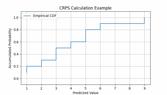
Example of CRPS calculation

CRPS and Skforecast¶

Skforecast provides different output options for probabilistic forecasting, two of which are:

• predict_bootstrapping: Returns multiple predicted values for each forecasted step. Each value is a variation of the forecast generated through bootstrapping. For a given step (i), (n) predictions are estimated.

• predict_quantile: Returns the estimated values for multiple quantiles. Internally, the forecaster uses predict_bootstrapping and then calculates the desired quantiles.

For both outputs, the CRPS (Continuous Ranked Probability Score) can be calculated to evaluate the forecasting performance of the model.

💡 Tip

For more examples on how to use probabilistic forecasting, check out the following articles:

• Probabilistic forecasting with machine learning
• Probabilistic forecasting: prediction intervals for multi-step time series forecasting
• Continuous Ranked Probability Score (CRPS) in probabilistic forecasting

CRPS from a sample of predictions¶

The Continuous Ranked Probability Score (CRPS) is calculated by comparing the empirical cumulative distribution function (ECDF) of the forecasted values to the step function CDF of the true value. When the available information consists of the true value (y_true) and a sample of predictions (y_pred), the CRPS can be calculated by following these steps:

1. Generate the Empirical Cumulative Distribution Function (ECDF) of the predictions:

   • Sort the predictions.
   • Use each sorted prediction as a step in the ECDF.

2. Generate the Cumulative Distribution Function (CDF) of the true value:

   • Since there is only a single true value, this is represented as a step function that jumps from 0 to 1 at the observed value (y_true).

3. Calculate the CRPS by integrating the area between both curves:

   • Create a grid of values to evaluate the ECDF. This grid is the combination of the predictions and the true value.
   • Compute the squared differences between the forecasted ECDF and the true CDF, and then summing the areas between the two curves.

In [1]:

# Libraries
# ======================================================================================
import pandas as pd
import numpy as np
from skforecast.metrics import crps_from_predictions
from skforecast.metrics import crps_from_quantiles
from scipy.interpolate import interp1d
import properscoring as ps
from CRPS import CRPS
from pymc_marketing.metrics import crps

# Libraries # ====================================================================================== import pandas as pd import numpy as np from skforecast.metrics import crps_from_predictions from skforecast.metrics import crps_from_quantiles from scipy.interpolate import interp1d import properscoring as ps from CRPS import CRPS from pymc_marketing.metrics import crps

WARNING (pytensor.configdefaults): g++ not detected!  PyTensor will be unable to compile C-implementations and will default to Python. Performance may be severely degraded. To remove this warning, set PyTensor flags cxx to an empty string.

In [2]:

# Simulate data: true value and and array of 100 predicted values for the same true value
# ======================================================================================
y_true = 500
y_pred = np.random.normal(500, 10, 100)
crps_from_predictions(y_true, y_pred)

# Simulate data: true value and and array of 100 predicted values for the same true value # ====================================================================================== y_true = 500 y_pred = np.random.normal(500, 10, 100) crps_from_predictions(y_true, y_pred)

Out[2]:

2.1767579851785803

The result of skforecast.metrics.crps_from_predictions is compared with other implemented functions in the properscoring, CRPS and pymc_marketing libraries.

In [3]:

# properscoring, CRPS, pymc-mar
# ==============================================================================
print(f"properscoring : {ps.crps_ensemble(y_true, y_pred)}")
print(f"CRPS          : {CRPS(y_pred, y_true).compute()[0]}")
print(f"pymc-marketing: {crps(y_true, y_pred.reshape(-1, 1))}")

# properscoring, CRPS, pymc-mar # ============================================================================== print(f"properscoring : {ps.crps_ensemble(y_true, y_pred)}") print(f"CRPS : {CRPS(y_pred, y_true).compute()[0]}") print(f"pymc-marketing: {crps(y_true, y_pred.reshape(-1, 1))}")

properscoring : 2.1767579851785785
CRPS          : 2.1767579851785803
pymc-marketing: 2.1767579851785808

When forecasting multiple steps, the CRPS can be calculated for each step and then averaged to provide a summary measure of the model's performance.

In [4]:

# CRPS for multiple steps
# ==============================================================================
rng = np.random.default_rng(123)
n_steps = 40
n_bootstraps = 100
predictions = pd.DataFrame({
    'y_true': rng.normal(100, 10, n_steps),
    'y_pred': [rng.normal(5, 5, n_bootstraps) for _ in range(n_steps)]
})

predictions['crps_from_predictions'] = predictions.apply(lambda x: crps_from_predictions(x['y_true'], x['y_pred']), axis=1)
predictions['properscoring'] = predictions.apply(lambda x: ps.crps_ensemble(x['y_true'], x['y_pred']), axis=1)
predictions['CRPS'] = predictions.apply(lambda x: CRPS(x['y_pred'], x['y_true']).compute()[0], axis=1)
predictions['pymc_marqueting'] = predictions.apply(lambda x: crps(x['y_true'], x['y_pred'].reshape(-1, 1)), axis=1)
display(predictions.head())

assert np.allclose(predictions['properscoring'], predictions['CRPS'])
assert np.allclose(predictions['properscoring'], predictions['pymc_marqueting'])
assert np.allclose(predictions['crps_from_predictions'], predictions['properscoring'])

# CRPS for multiple steps # ============================================================================== rng = np.random.default_rng(123) n_steps = 40 n_bootstraps = 100 predictions = pd.DataFrame({ 'y_true': rng.normal(100, 10, n_steps), 'y_pred': [rng.normal(5, 5, n_bootstraps) for _ in range(n_steps)] }) predictions['crps_from_predictions'] = predictions.apply(lambda x: crps_from_predictions(x['y_true'], x['y_pred']), axis=1) predictions['properscoring'] = predictions.apply(lambda x: ps.crps_ensemble(x['y_true'], x['y_pred']), axis=1) predictions['CRPS'] = predictions.apply(lambda x: CRPS(x['y_pred'], x['y_true']).compute()[0], axis=1) predictions['pymc_marqueting'] = predictions.apply(lambda x: crps(x['y_true'], x['y_pred'].reshape(-1, 1)), axis=1) display(predictions.head()) assert np.allclose(predictions['properscoring'], predictions['CRPS']) assert np.allclose(predictions['properscoring'], predictions['pymc_marqueting']) assert np.allclose(predictions['crps_from_predictions'], predictions['properscoring'])

	y_true	y_pred	crps_from_predictions	properscoring	CRPS	pymc_marqueting
0	90.108786	[8.640637789445714, -1.3080015845984816, 12.14...	82.100538	82.100538	82.100538	82.100538
1	96.322133	[3.1678558225107745, 6.737363230274925, 5.6735...	88.410864	88.410864	88.410864	88.410864
2	112.879253	[6.709160916434245, 10.896201858093296, 0.9120...	105.460630	105.460630	105.460630	105.460630
3	101.939744	[14.521434285699028, 1.1295876122380442, 15.13...	94.259885	94.259885	94.259885	94.259885
4	109.202309	[13.80532539228533, 5.482203757147254, 6.46324...	101.908526	101.908526	101.908526	101.908526

In [5]:

# Average CRPS
# ==============================================================================
mean_crps = predictions[['crps_from_predictions', 'properscoring', 'CRPS', 'pymc_marqueting']].mean()
mean_crps

# Average CRPS # ============================================================================== mean_crps = predictions[['crps_from_predictions', 'properscoring', 'CRPS', 'pymc_marqueting']].mean() mean_crps

Out[5]:

crps_from_predictions    93.974753
properscoring            93.974753
CRPS                     93.974753
pymc_marqueting          93.974753
dtype: float64

CRPS from quantiles¶

A quantile is a value that divides a data set into intervals, with a specific percentage of the data lying below it. Essentially, it is a point on the cumulative distribution function (CDF) that represents a threshold at which a given proportion of the data is less than or equal to that value.

For example, the 40th percentile (or 0.4 quantile) is the value below which 40% of the data points fall. To find it, you would examine the CDF, which shows the cumulative proportion of the data as you move along the values of the data set. The 0.4 quantile corresponds to the point where the CDF reaches 0.4 on the vertical axis, indicating that 40% of the data lies at or below this value.

This relationship between quantiles and the CDF means that, given several quantile values, it is possible to reconstruct the CDF. This is essential for calculating the Continuous Ranked Probability Score (CRPS), which measures the accuracy of probabilistic forecasts by comparing how well the predicted distribution matches the true value.

Given a set of quantiles, their associated probabilities, and the true value, the CRPS can be calculated as follows:

1. Construct the Empirical Cumulative Distribution Function (ECDF) using the quantiles and their corresponding probabilities.

2. Generate the CDF for the true value: Since the true value is a single point, its CDF is represented as a step function that jumps from 0 to 1 at the observed value.

3. Calculate the CRPS as the squared diference between the two curves.

In [6]:

# CRPS score from quantiles
# ==============================================================================
y_true = 3.0

quantile_levels = np.array([
    0.00, 0.025, 0.05, 0.10, 0.15, 0.20, 0.25, 0.30, 0.35, 0.40, 0.45, 0.50, 0.55,
    0.60, 0.65, 0.70, 0.75, 0.80, 0.85, 0.90, 0.95, 0.975, 1.00
])
pred_quantiles = np.array([
    0.1, 1.0, 1.5, 2.0, 2.5, 3.0, 3.5, 4.0, 4.5, 5.0, 5.5, 6.0, 6.5, 7.0, 7.5,
    8.0, 8.5, 9.0, 9.5, 10.0, 10.5, 11.0, 11.5
])

crps_from_quantiles(y_true, pred_quantiles, quantile_levels)

# CRPS score from quantiles # ============================================================================== y_true = 3.0 quantile_levels = np.array([ 0.00, 0.025, 0.05, 0.10, 0.15, 0.20, 0.25, 0.30, 0.35, 0.40, 0.45, 0.50, 0.55, 0.60, 0.65, 0.70, 0.75, 0.80, 0.85, 0.90, 0.95, 0.975, 1.00 ]) pred_quantiles = np.array([ 0.1, 1.0, 1.5, 2.0, 2.5, 3.0, 3.5, 4.0, 4.5, 5.0, 5.5, 6.0, 6.5, 7.0, 7.5, 8.0, 8.5, 9.0, 9.5, 10.0, 10.5, 11.0, 11.5 ]) crps_from_quantiles(y_true, pred_quantiles, quantile_levels)

Out[6]:

1.7339183102042313

Again, results are compared versus the properscoring package. In this case, a warapper function is used to calculate the CRPS score from the predicted quantiles using crps_quadrature.

In [7]:

def crps_from_quantiles_properscoring(y_true, predicted_quantiles, quantile_levels):
    """
    Calculate the Continuous Ranked Probability Score (CRPS) for a given true value
    and predicted quantiles using the function crps_quadrature from the properscoring
    library.

    Parameters
    ----------
    y_true : float
        The true value of the random variable.
    predicted_quantiles : np.array
        The predicted quantile values.
    quantile_levels : np.array
        The quantile levels corresponding to the predicted quantiles.

    Returns
    -------
    float
        The CRPS score.
    """
    if len(predicted_quantiles) != len(quantile_levels):
        raise ValueError(
            "The number of predicted quantiles and quantile levels must be equal."
        )
    
    # Ensure predicted_quantiles are sorted
    sort_idx = np.argsort(predicted_quantiles)
    predicted_quantiles = predicted_quantiles[sort_idx]
    quantile_levels = quantile_levels[sort_idx]

    def empirical_cdf(x):
        # Interpolate between quantile levels and quantile values
        cdf_func = interp1d(
            predicted_quantiles,
            quantile_levels,
            bounds_error=False,
            fill_value=(0.0, 1.0),
        )
        return cdf_func(x)

    # Integration bounds
    xmin = np.min(predicted_quantiles) * 0.9
    xmax = np.max(predicted_quantiles) * 1.1

    # Compute CRPS
    crps = ps.crps_quadrature(np.array([y_true]), empirical_cdf, xmin, xmax)

    return crps[0]


crps_from_quantiles_properscoring(y_true, pred_quantiles, quantile_levels)

def crps_from_quantiles_properscoring(y_true, predicted_quantiles, quantile_levels): """ Calculate the Continuous Ranked Probability Score (CRPS) for a given true value and predicted quantiles using the function crps_quadrature from the properscoring library. Parameters ---------- y_true : float The true value of the random variable. predicted_quantiles : np.array The predicted quantile values. quantile_levels : np.array The quantile levels corresponding to the predicted quantiles. Returns ------- float The CRPS score. """ if len(predicted_quantiles) != len(quantile_levels): raise ValueError( "The number of predicted quantiles and quantile levels must be equal." ) # Ensure predicted_quantiles are sorted sort_idx = np.argsort(predicted_quantiles) predicted_quantiles = predicted_quantiles[sort_idx] quantile_levels = quantile_levels[sort_idx] def empirical_cdf(x): # Interpolate between quantile levels and quantile values cdf_func = interp1d( predicted_quantiles, quantile_levels, bounds_error=False, fill_value=(0.0, 1.0), ) return cdf_func(x) # Integration bounds xmin = np.min(predicted_quantiles) * 0.9 xmax = np.max(predicted_quantiles) * 1.1 # Compute CRPS crps = ps.crps_quadrature(np.array([y_true]), empirical_cdf, xmin, xmax) return crps[0] crps_from_quantiles_properscoring(y_true, pred_quantiles, quantile_levels)

Out[7]:

1.7342500001706027

Results are similar but not identical. This may be due to differences in the implementation of the CRPS calculation or the numerical methods used to approximate the integral. The skforecast team is working on validating the implementation of the CRPS function in the library.