Probabilistic forecasting: prediction intervals and prediction distribution¶

When trying to anticipate future values, most forecasting models focus on predicting the most likely value, which is called point-forecasting. Although knowing the expected value of a time series is useful for most business cases, this type of forecasting does not provide any information about the model's confidence or the prediction's uncertainty.

Probabilistic forecasting, as opposed to point-forecasting, is a family of techniques that enable the prediction of the expected distribution of the outcome, rather than a single future value. This type of forecasting provides much richer information, as it reports the range of probable values into which the true value may fall, allowing the estimation of prediction intervals.

A prediction interval is the interval within which the true value of the response variable is expected to be found with a given probability. There are multiple ways to estimate prediction intervals, most of which require that the residuals (errors) of the model follow a normal distribution. However, when this assumption cannot be made, two commonly used alternatives are bootstrapping and quantile regression.

To illustrate how skforecast enables the estimation of prediction intervals for multi-step forecasting, examples attempting to predict energy demand for a 7-day horizon are provided. Two strategies are showcased:

• Prediction intervals based on bootstrapped residuals.

• Prediction intervals based on quantile regression.

  Warning

As Rob J Hyndman explains in his blog, in real-world problems, almost all prediction intervals are too narrow. For example, nominal 95% intervals may only provide coverage between 71% and 87%. This is a well-known phenomenon and arises because they do not account for all sources of uncertainty. With forecasting models, there are at least four sources of uncertainty:

• The random error term
• The parameter estimates
• The choice of model for the historical data
• The continuation of the historical data generating process into the future

When producing prediction intervals for time series models, generally only the first of these sources is taken into account. Therefore, it is advisable to use test data to validate the empirical coverage of the interval and not solely rely on the expected coverage.

Predicting distribution and intervals using bootstrapped residuals¶

The error of a one-step-ahead forecast is defined as the difference between the actual value and the predicted value ($e_t=y_t-{\hat{y}}_{t|t-1}$). By assuming that future errors will be similar to past errors, it is possible to simulate different predictions by taking samples from the collection of errors previously seen in the past (i.e., the residuals) and adding them to the predictions.

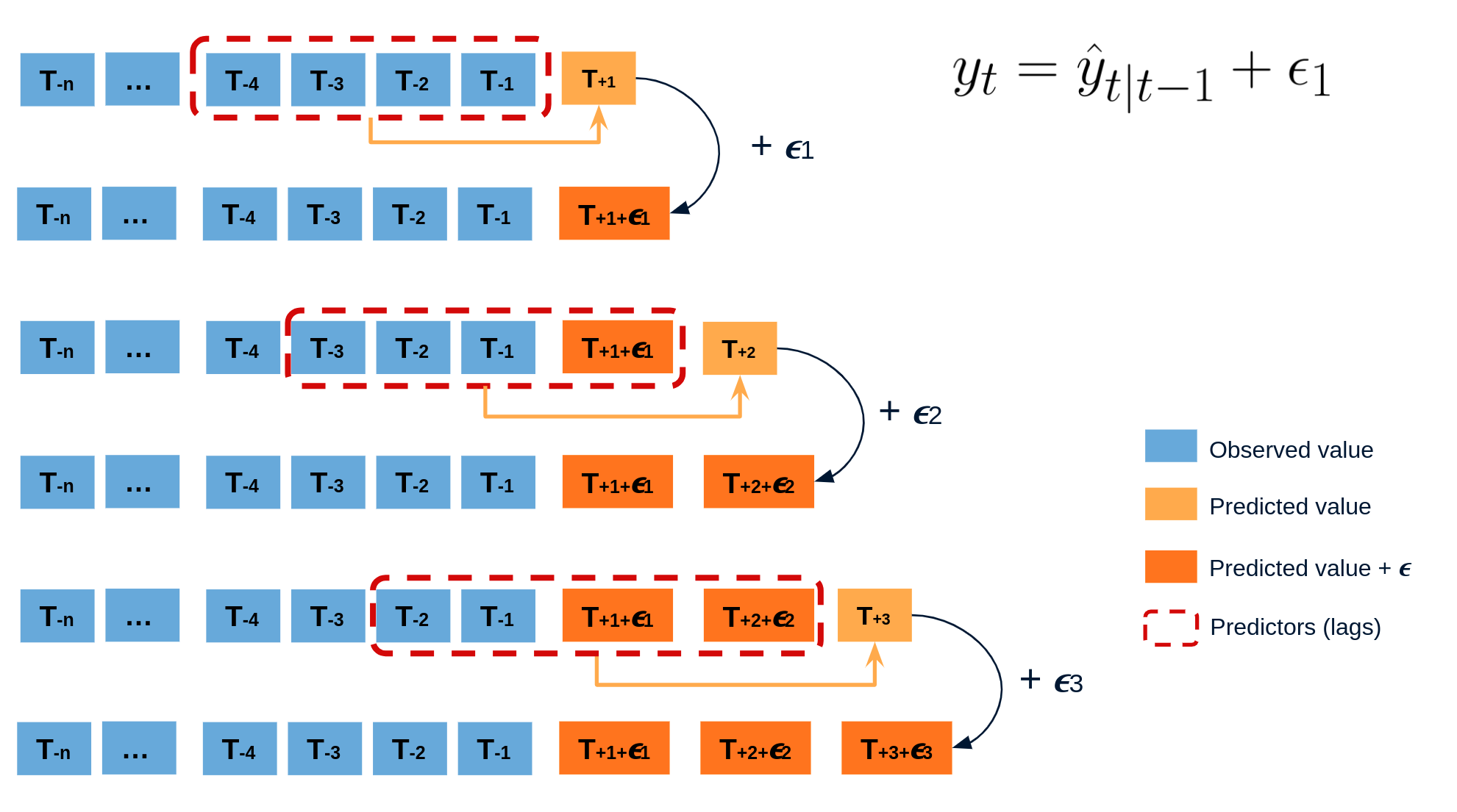
Diagram bootstrapping prediction process.

Repeatedly performing this process creates a collection of slightly different predictions, which represent the distribution of possible outcomes due to the expected variance in the forecasting process.

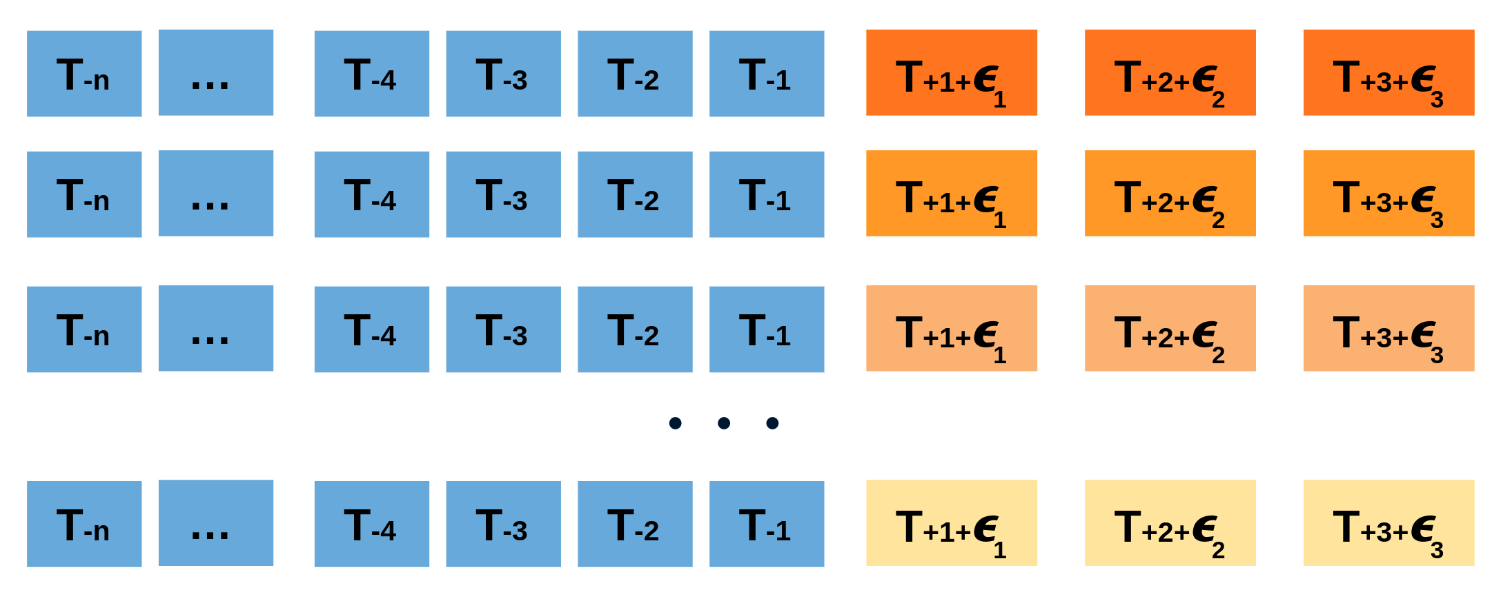
Bootstrapping predictions.

Using the outcome of the bootstrapping process, prediction intervals can be computed by calculating the $\alpha /2$ and $1-\alpha /2$ percentiles at each forecasting horizon.

Alternatively, it is also possible to fit a parametric distribution for each forecast horizon.

One of the main advantages of this strategy is that it requires only a single model to estimate any interval. However, performing hundreds or thousands of bootstrapping iterations can be computationally expensive and may not always be feasible.

Probabilistic prediction methods¶

In skforecast, all forecasters have three different methods that allow for probabilistic forecasting:

• predict_bootstrapping: this method generates multiple forecasting predictions through a bootstrapping process. By sampling from a collection of past observed errors (the residuals), each bootstrapping iteration generates a different set of predictions. The output is a pandas DataFrame with one row for each predicted step and one column for each bootstrapping iteration.

• predict_intervals: this method estimates quantile predictions intervals using the values generated with predict_bootstrapping.

• predict_quantiles: this method estimates a list of quantile predictions using the values generated with predict_bootstrapping.

• predict_dist: this method fits a parametric distribution using the values generated with predict_bootstrapping. Any of the continuous distributions available in scipy.stats can be used.

  Tip

The following example shows how to use these methods with a ForecasterAutoreg, but note that this works for all other types of Forecasters as well.

Libraries¶

In [1]:

# Data processing
# ==============================================================================
import numpy as np
import pandas as pd

# Plots
# ==============================================================================
import matplotlib.pyplot as plt
import matplotlib.ticker as ticker
plt.style.use('seaborn-v0_8-darkgrid')

# Modelling and Forecasting
# ==============================================================================
from skforecast.ForecasterAutoreg import ForecasterAutoreg
from skforecast.ForecasterAutoregDirect import ForecasterAutoregDirect
from skforecast.plot import plot_prediction_distribution
from skforecast.model_selection import backtesting_forecaster
from skforecast.model_selection import grid_search_forecaster
from lightgbm import LGBMRegressor
from sklearn.metrics import mean_pinball_loss
from skforecast.exceptions import LongTrainingWarning

# Configuration
# ==============================================================================
import warnings
warnings.filterwarnings('once')

# Data processing # ============================================================================== import numpy as np import pandas as pd # Plots # ============================================================================== import matplotlib.pyplot as plt import matplotlib.ticker as ticker plt.style.use('seaborn-v0_8-darkgrid') # Modelling and Forecasting # ============================================================================== from skforecast.ForecasterAutoreg import ForecasterAutoreg from skforecast.ForecasterAutoregDirect import ForecasterAutoregDirect from skforecast.plot import plot_prediction_distribution from skforecast.model_selection import backtesting_forecaster from skforecast.model_selection import grid_search_forecaster from lightgbm import LGBMRegressor from sklearn.metrics import mean_pinball_loss from skforecast.exceptions import LongTrainingWarning # Configuration # ============================================================================== import warnings warnings.filterwarnings('once')

Data¶

In [2]:

# Data download
# ==============================================================================
url = (
       'https://raw.githubusercontent.com/JoaquinAmatRodrigo/skforecast/master/'
       'data/vic_elec.csv'
)
data = pd.read_csv(url, sep=',')

# Data preparation (aggregation at daily level)
# ==============================================================================
data['Time'] = pd.to_datetime(data['Time'], format='%Y-%m-%dT%H:%M:%SZ')
data = data.set_index('Time')
data = data.asfreq('30min')
data = data.sort_index()
data = data.drop(columns='Date')
data = data.resample(rule='D', closed='left', label ='right')\
       .agg({'Demand': 'sum', 'Temperature': 'mean', 'Holiday': 'max'})

data.head(3)

# Data download # ============================================================================== url = ( 'https://raw.githubusercontent.com/JoaquinAmatRodrigo/skforecast/master/' 'data/vic_elec.csv' ) data = pd.read_csv(url, sep=',') # Data preparation (aggregation at daily level) # ============================================================================== data['Time'] = pd.to_datetime(data['Time'], format='%Y-%m-%dT%H:%M:%SZ') data = data.set_index('Time') data = data.asfreq('30min') data = data.sort_index() data = data.drop(columns='Date') data = data.resample(rule='D', closed='left', label ='right')\ .agg({'Demand': 'sum', 'Temperature': 'mean', 'Holiday': 'max'}) data.head(3)

Out[2]:

	Demand	Temperature	Holiday
Time
2012-01-01	82531.745918	21.047727	True
2012-01-02	227778.257304	26.578125	True
2012-01-03	275490.988882	31.751042	True

In [3]:

# Split data into train-validation-test
# ==============================================================================
data = data.loc['2012-01-01 00:00:00': '2014-12-30 23:00:00']
end_train = '2013-12-31 23:59:00'
end_validation = '2014-9-30 23:59:00'
data_train = data.loc[: end_train, :].copy()
data_val   = data.loc[end_train:end_validation, :].copy()
data_test  = data.loc[end_validation:, :].copy()

print(
    f"Train dates      : {data_train.index.min()} --- {data_train.index.max()}"
    f"  (n={len(data_train)})"
)
print(
    f"Validation dates : {data_val.index.min()} --- {data_val.index.max()}"
    f"  (n={len(data_val)})"
)
print(
    f"Test dates       : {data_test.index.min()} --- {data_test.index.max()}"
    f"  (n={len(data_test)})"
)

# Split data into train-validation-test # ============================================================================== data = data.loc['2012-01-01 00:00:00': '2014-12-30 23:00:00'] end_train = '2013-12-31 23:59:00' end_validation = '2014-9-30 23:59:00' data_train = data.loc[: end_train, :].copy() data_val = data.loc[end_train:end_validation, :].copy() data_test = data.loc[end_validation:, :].copy() print( f"Train dates : {data_train.index.min()} --- {data_train.index.max()}" f" (n={len(data_train)})" ) print( f"Validation dates : {data_val.index.min()} --- {data_val.index.max()}" f" (n={len(data_val)})" ) print( f"Test dates : {data_test.index.min()} --- {data_test.index.max()}" f" (n={len(data_test)})" )

Train dates      : 2012-01-01 00:00:00 --- 2013-12-31 00:00:00  (n=731)
Validation dates : 2014-01-01 00:00:00 --- 2014-09-30 00:00:00  (n=273)
Test dates       : 2014-10-01 00:00:00 --- 2014-12-30 00:00:00  (n=91)

In [4]:

# Plot time series partition
# ==============================================================================
fig, ax = plt.subplots(figsize=(9, 3))
data_train['Demand'].plot(label='train', ax=ax)
data_val['Demand'].plot(label='validation', ax=ax)
data_test['Demand'].plot(label='test', ax=ax)
ax.yaxis.set_major_formatter(ticker.EngFormatter())
ax.set_ylim(bottom=160_000)
ax.set_ylabel('MW')
ax.set_xlabel('')
ax.set_title('Energy demand')
ax.legend();

# Plot time series partition # ============================================================================== fig, ax = plt.subplots(figsize=(9, 3)) data_train['Demand'].plot(label='train', ax=ax) data_val['Demand'].plot(label='validation', ax=ax) data_test['Demand'].plot(label='test', ax=ax) ax.yaxis.set_major_formatter(ticker.EngFormatter()) ax.set_ylim(bottom=160_000) ax.set_ylabel('MW') ax.set_xlabel('') ax.set_title('Energy demand') ax.legend();

Probabilistic forecasting¶

In [5]:

# Create and train a ForecasterAutoreg
# ==============================================================================
forecaster = ForecasterAutoreg(
                 regressor = LGBMRegressor(
                                 learning_rate = 0.01,
                                 max_depth     = 10,
                                 n_estimators  = 500,
                                 random_state  = 123
                             ),
                 lags      = 7
             )

forecaster.fit(y=data.loc[end_train:end_validation, 'Demand'])
forecaster

# Create and train a ForecasterAutoreg # ============================================================================== forecaster = ForecasterAutoreg( regressor = LGBMRegressor( learning_rate = 0.01, max_depth = 10, n_estimators = 500, random_state = 123 ), lags = 7 ) forecaster.fit(y=data.loc[end_train:end_validation, 'Demand']) forecaster

Out[5]:

================= 
ForecasterAutoreg 
================= 
Regressor: LGBMRegressor(learning_rate=0.01, max_depth=10, n_estimators=500,
              random_state=123) 
Lags: [1 2 3 4 5 6 7] 
Transformer for y: None 
Transformer for exog: None 
Window size: 7 
Weight function included: False 
Differentiation order: None 
Exogenous included: False 
Type of exogenous variable: None 
Exogenous variables names: None 
Training range: [Timestamp('2014-01-01 00:00:00'), Timestamp('2014-09-30 00:00:00')] 
Training index type: DatetimeIndex 
Training index frequency: D 
Regressor parameters: {'boosting_type': 'gbdt', 'class_weight': None, 'colsample_bytree': 1.0, 'importance_type': 'split', 'learning_rate': 0.01, 'max_depth': 10, 'min_child_samples': 20, 'min_child_weight': 0.001, 'min_split_gain': 0.0, 'n_estimators': 500, 'n_jobs': -1, 'num_leaves': 31, 'objective': None, 'random_state': 123, 'reg_alpha': 0.0, 'reg_lambda': 0.0, 'silent': 'warn', 'subsample': 1.0, 'subsample_for_bin': 200000, 'subsample_freq': 0} 
fit_kwargs: {} 
Creation date: 2023-11-15 19:20:18 
Last fit date: 2023-11-15 19:20:18 
Skforecast version: 0.11.0 
Python version: 3.10.11 
Forecaster id: None 

Predict Bootstraping¶

Once the Forecaster has been trained, the method predict_bootstraping can be use to simulate n_boot values of the forecasting distribution.

In [6]:

# Predict 10 different forecasting sequences of 7 steps each using bootstrapping
# ==============================================================================
boot_predictions = forecaster.predict_bootstrapping(steps=7, n_boot=10)
boot_predictions

# Predict 10 different forecasting sequences of 7 steps each using bootstrapping # ============================================================================== boot_predictions = forecaster.predict_bootstrapping(steps=7, n_boot=10) boot_predictions

Out[6]:

	pred_boot_0	pred_boot_1	pred_boot_2	pred_boot_3	pred_boot_4	pred_boot_5	pred_boot_6	pred_boot_7	pred_boot_8	pred_boot_9
2014-10-01	208783.097577	204764.999003	201367.203420	212280.661192	204622.100582	202889.246579	210078.609982	210151.742392	200990.348257	203137.232359
2014-10-02	212340.130913	208320.030667	217221.147681	209996.152477	218464.949614	212545.697772	212061.596039	216579.376162	226902.326444	212847.017644
2014-10-03	221380.131363	223890.630246	224625.204840	207260.018970	206099.826214	288939.369743	220085.831843	229514.853352	230476.360893	224059.729506
2014-10-04	209943.773973	212946.528553	200027.296792	203592.696069	194120.730680	262225.653280	212516.896678	222042.271003	215236.033624	222487.580478
2014-10-05	193372.607408	177195.227257	194351.934752	206606.909536	202654.435499	297740.735825	192454.576530	199372.141645	208527.690318	197830.624380
2014-10-06	199626.367544	203338.054671	207145.334747	208993.695577	204766.177714	258050.416951	184903.916795	201473.420885	204790.425542	183312.907014
2014-10-07	201546.003371	212477.910879	209639.468951	204102.852012	225036.945159	257847.869040	197235.769115	196990.134684	200007.936217	207116.299541

Using a ridge plot is a useful way to visualize the uncertainty of a forecasting model. This plot estimates a kernel density for each step by using the bootstrapped predictions.

In [7]:

# Ridge plot of bootstrapping predictions
# ==============================================================================
_ = plot_prediction_distribution(boot_predictions, figsize=(7, 4))

# Ridge plot of bootstrapping predictions # ============================================================================== _ = plot_prediction_distribution(boot_predictions, figsize=(7, 4))

Predict Interval¶

In most cases, the user is interested in a specific interval rather than the entire bootstrapping simulation matrix. To address this need, skforecast provides the predict_interval method. This method internally uses predict_bootstrapping to obtain the bootstrapping matrix and estimates the upper and lower quantiles for each step, thus providing the user with the desired prediction intervals.

In [8]:

# Predict intervals for next 7 steps, quantiles 10th and 90th
# ==============================================================================
predictions = forecaster.predict_interval(steps=7, interval=[10, 90], n_boot=1000)
predictions

# Predict intervals for next 7 steps, quantiles 10th and 90th # ============================================================================== predictions = forecaster.predict_interval(steps=7, interval=[10, 90], n_boot=1000) predictions

Out[8]:

	pred	lower_bound	upper_bound
2014-10-01	205723.923923	195483.862851	214883.472075
2014-10-02	215167.163121	204160.738452	225623.750301
2014-10-03	225144.443075	212599.136391	237675.514362
2014-10-04	211406.440681	196863.841123	234950.293307
2014-10-05	194848.766987	185544.868289	225497.131653
2014-10-06	201901.819903	188334.486578	226720.998742
2014-10-07	208648.526025	191797.716429	231948.852094

Predict Quantile¶

This method operates identically to predict_interval, with the added feature of enabling users to define a specific list of quantiles for estimation at each step. It's important to remember that these quantiles should be specified within the range of 0 to 1.

In [9]:

# Predict quantiles for next 7 steps, quantiles 5th, 25th, 75th and 95th
# ==============================================================================
predictions = forecaster.predict_quantiles(steps=7, quantiles=[0.05, 0.25, 0.75, 0.95], n_boot=1000)
predictions

# Predict quantiles for next 7 steps, quantiles 5th, 25th, 75th and 95th # ============================================================================== predictions = forecaster.predict_quantiles(steps=7, quantiles=[0.05, 0.25, 0.75, 0.95], n_boot=1000) predictions

Out[9]:

	q_0.05	q_0.25	q_0.75	q_0.95
2014-10-01	190931.232112	201367.203420	209262.858754	217730.216823
2014-10-02	200073.450004	209983.877484	219323.939792	240417.202430
2014-10-03	208422.554331	218572.814092	230091.464603	251383.795523
2014-10-04	192618.644753	204251.785931	222408.098868	256285.360096
2014-10-05	181143.759693	191499.233675	207377.126997	255789.774545
2014-10-06	184887.453266	194613.761232	208546.550156	257237.948263
2014-10-07	187384.716314	198277.712914	212038.622323	256921.642212

Predict Distribution¶

The intervals estimated so far are distribution-free, which means that no assumptions are made about a particular distribution. The predict_dist method in skforecast allows fitting a parametric distribution to the bootstrapped prediction samples obtained with predict_bootstrapping. This is useful when there is reason to believe that the forecast errors follow a particular distribution, such as the normal distribution or the student's t-distribution. The predict_dist method allows the user to specify any continuous distribution from the scipy.stats module.

In [10]:

# Predict the parameters of a normal distribution for the next 7 steps
# ==============================================================================
from scipy.stats import norm

predictions = forecaster.predict_dist(steps=7, distribution=norm, n_boot=1000)
predictions

# Predict the parameters of a normal distribution for the next 7 steps # ============================================================================== from scipy.stats import norm predictions = forecaster.predict_dist(steps=7, distribution=norm, n_boot=1000) predictions

Out[10]:

	loc	scale
2014-10-01	205374.632063	12290.061732
2014-10-02	215791.488070	13607.935838
2014-10-03	225631.039103	14206.970100
2014-10-04	215210.987777	18980.776421
2014-10-05	202613.715687	19980.302998
2014-10-06	205391.493409	19779.732794
2014-10-07	208579.269999	18950.289467

Backtesting with prediction intervals¶

A backtesting process can be applied to evaluate the performance of the forecaster over a period of time, for example on test data, and calculate the actual coverage of the estimated range.

In [11]:

# Backtesting on test data 
# ==============================================================================
metric, predictions = backtesting_forecaster(
                          forecaster            = forecaster,
                          y                     = data['Demand'],
                          steps                 = 7,
                          metric                = 'mean_squared_error',
                          initial_train_size    = len(data_train) + len(data_val),
                          fixed_train_size      = True,
                          gap                   = 0,
                          allow_incomplete_fold = True,
                          refit                 = True,
                          interval              = [10, 90],
                          n_boot                = 1000,
                          random_state          = 123,
                          verbose               = False,
                          show_progress         = True
                      )
predictions.head(4)

# Backtesting on test data # ============================================================================== metric, predictions = backtesting_forecaster( forecaster = forecaster, y = data['Demand'], steps = 7, metric = 'mean_squared_error', initial_train_size = len(data_train) + len(data_val), fixed_train_size = True, gap = 0, allow_incomplete_fold = True, refit = True, interval = [10, 90], n_boot = 1000, random_state = 123, verbose = False, show_progress = True ) predictions.head(4)

  0%|          | 0/13 [00:00<?, ?it/s]

Out[11]:

	pred	lower_bound	upper_bound
2014-10-01	223264.432587	214633.692784	231376.785240
2014-10-02	233596.210854	223051.862727	244752.538248
2014-10-03	242653.671597	226947.654906	258361.695192
2014-10-04	220842.603128	209967.438912	236404.408845

In [12]:

# Plot
# ==============================================================================
fig, ax = plt.subplots(figsize=(7, 3))
data.loc[end_validation:, 'Demand'].plot(ax=ax, label='Demand')
ax.fill_between(
    predictions.index,
    predictions['lower_bound'],
    predictions['upper_bound'],
    color = 'deepskyblue',
    alpha = 0.3,
    label = '80% interval'
)
ax.yaxis.set_major_formatter(ticker.EngFormatter())
ax.set_ylabel('MW')
ax.set_xlabel('')
ax.set_title('Energy demand forecast')
ax.legend();

# Plot # ============================================================================== fig, ax = plt.subplots(figsize=(7, 3)) data.loc[end_validation:, 'Demand'].plot(ax=ax, label='Demand') ax.fill_between( predictions.index, predictions['lower_bound'], predictions['upper_bound'], color = 'deepskyblue', alpha = 0.3, label = '80% interval' ) ax.yaxis.set_major_formatter(ticker.EngFormatter()) ax.set_ylabel('MW') ax.set_xlabel('') ax.set_title('Energy demand forecast') ax.legend();

In [13]:

# Interval coverage on test data
# ==============================================================================
inside_interval = np.where(
                      (data.loc[predictions.index, 'Demand'] >= predictions['lower_bound']) & \
                      (data.loc[predictions.index, 'Demand'] <= predictions['upper_bound']),
                      True,
                      False
                  )

coverage = inside_interval.mean()
print(f"Coverage of the predicted interval on test data: {100 * coverage}")

# Interval coverage on test data # ============================================================================== inside_interval = np.where( (data.loc[predictions.index, 'Demand'] >= predictions['lower_bound']) & \ (data.loc[predictions.index, 'Demand'] <= predictions['upper_bound']), True, False ) coverage = inside_interval.mean() print(f"Coverage of the predicted interval on test data: {100 * coverage}")

Coverage of the predicted interval on test data: 65.93406593406593

The coverage of the predicted interval is much lower than expected (80%).

Prediction with out-sample residuals¶

By default, the training residuals are used to create the prediction intervals. However, this is not the most recommended option as the estimated interval tends to be too narrow. This is because the model's performance on training data is usually better than on new observations, leading to smaller residuals and, in turn, narrower prediction intervals.

To overcome this issue, it is advisable to use other residuals, such as those obtained from a validation set. This can be achieved by storing the new residuals inside the forecaster using the set_out_sample_residuals method.

In [14]:

# Backtesting using validation data
# ==============================================================================
metric, backtest_predictions = backtesting_forecaster(
                                   forecaster         = forecaster,
                                   y                  = data.loc[:end_validation, 'Demand'],
                                   initial_train_size = len(data_train),
                                   steps              = 7,
                                   refit              = True,
                                   metric             = 'mean_squared_error',
                                   verbose            = False,
                                   show_progress      = True
                               )

# Calculate residuals in validation data
# ==============================================================================
residuals = (data_val['Demand'] - backtest_predictions['pred']).to_numpy()
residuals[:5]

# Backtesting using validation data # ============================================================================== metric, backtest_predictions = backtesting_forecaster( forecaster = forecaster, y = data.loc[:end_validation, 'Demand'], initial_train_size = len(data_train), steps = 7, refit = True, metric = 'mean_squared_error', verbose = False, show_progress = True ) # Calculate residuals in validation data # ============================================================================== residuals = (data_val['Demand'] - backtest_predictions['pred']).to_numpy() residuals[:5]

  0%|          | 0/39 [00:00<?, ?it/s]

Out[14]:

array([-16084.02669559, -14168.47600418,  -4416.31618072, -15101.78356121,
       -31133.70782794])

Once the residuals of the validation set are calculated, they can be stored inside the forecaster. This allows the forecaster to use the out-of-sample residuals for prediction interval calculation instead of the default in-sample residuals. By doing so, the estimated prediction intervals will be less optimistic and more representative of the performance of the model on new observations.

In [15]:

# Set out-sample residuals
# ==============================================================================
forecaster.set_out_sample_residuals(residuals=residuals)

# Set out-sample residuals # ============================================================================== forecaster.set_out_sample_residuals(residuals=residuals)

Once the new residuals have been added to the forecaster, use in_sample_residuals = False when calling the prediction methods.

In [16]:

# Predict intervals using out-sample residuals
# ==============================================================================
forecaster.predict_interval(
    steps               = 7, 
    interval            = [10, 90], 
    n_boot              = 1000,
    in_sample_residuals = False
)

# Predict intervals using out-sample residuals # ============================================================================== forecaster.predict_interval( steps = 7, interval = [10, 90], n_boot = 1000, in_sample_residuals = False )

Out[16]:

	pred	lower_bound	upper_bound
2014-10-01	205723.923923	186442.948366	219301.240056
2014-10-02	215167.163121	193309.527919	237664.343916
2014-10-03	225144.443075	202621.185338	248592.853063
2014-10-04	211406.440681	190686.942976	252492.488196
2014-10-05	194848.766987	182470.870866	246304.519999
2014-10-06	201901.819903	183721.031607	243358.781198
2014-10-07	208648.526025	183541.873516	244359.947649

Also, a backtesting process can be applied to the test data with in_sample_residuals = False to use the out-of-sample residuals in the interval estimation.

In [17]:

# Backtesting using test data and out-sample residuals
# ==============================================================================
metric, predictions_2 = backtesting_forecaster(
                            forecaster          = forecaster,
                            y                   = data['Demand'],
                            initial_train_size  = len(data_train) + len(data_val),
                            steps               = 7,
                            refit               = True,
                            interval            = [10, 90],
                            n_boot              = 1000,
                            in_sample_residuals = False,
                            random_state        = 123,
                            metric              = 'mean_squared_error',
                            verbose             = False,
                            show_progress       = True
                        )

predictions_2.head(4)

# Backtesting using test data and out-sample residuals # ============================================================================== metric, predictions_2 = backtesting_forecaster( forecaster = forecaster, y = data['Demand'], initial_train_size = len(data_train) + len(data_val), steps = 7, refit = True, interval = [10, 90], n_boot = 1000, in_sample_residuals = False, random_state = 123, metric = 'mean_squared_error', verbose = False, show_progress = True ) predictions_2.head(4)

  0%|          | 0/13 [00:00<?, ?it/s]

Out[17]:

	pred	lower_bound	upper_bound
2014-10-01	223264.432587	203983.457029	236841.748720
2014-10-02	233596.210854	207273.919217	255429.172682
2014-10-03	242653.671597	211668.258043	265757.229322
2014-10-04	220842.603128	195869.206779	245921.530106

In [18]:

# Plot
# ==============================================================================
fig, ax = plt.subplots(figsize=(7, 4))
data.loc[end_validation:, 'Demand'].plot(ax=ax, label='Demand')
ax.fill_between(
    predictions.index,
    predictions['lower_bound'],
    predictions['upper_bound'],
    color = 'orange',
    alpha = 0.3,
    label = '80% interval in-sample residuals'
)
ax.fill_between(
    predictions_2.index,
    predictions_2['lower_bound'],
    predictions_2['upper_bound'],
    color = 'deepskyblue',
    alpha = 0.3,
    label = '80% interval out-sample residuals'
)
ax.yaxis.set_major_formatter(ticker.EngFormatter())
ax.set_ylabel('MW')
ax.set_xlabel('')
ax.set_title('Energy demand forecast')
ax.legend(fontsize=10);

# Plot # ============================================================================== fig, ax = plt.subplots(figsize=(7, 4)) data.loc[end_validation:, 'Demand'].plot(ax=ax, label='Demand') ax.fill_between( predictions.index, predictions['lower_bound'], predictions['upper_bound'], color = 'orange', alpha = 0.3, label = '80% interval in-sample residuals' ) ax.fill_between( predictions_2.index, predictions_2['lower_bound'], predictions_2['upper_bound'], color = 'deepskyblue', alpha = 0.3, label = '80% interval out-sample residuals' ) ax.yaxis.set_major_formatter(ticker.EngFormatter()) ax.set_ylabel('MW') ax.set_xlabel('') ax.set_title('Energy demand forecast') ax.legend(fontsize=10);

In [19]:

# Interval coverage on test data
# ==============================================================================
inside_interval = np.where(
                      (data.loc[predictions_2.index, 'Demand'] >= predictions_2['lower_bound']) & \
                      (data.loc[predictions_2.index, 'Demand'] <= predictions_2['upper_bound']),
                      True,
                      False
                  )

coverage = inside_interval.mean()
print(f"Coverage of the predicted interval on test data: {100 * coverage}")

# Interval coverage on test data # ============================================================================== inside_interval = np.where( (data.loc[predictions_2.index, 'Demand'] >= predictions_2['lower_bound']) & \ (data.loc[predictions_2.index, 'Demand'] <= predictions_2['upper_bound']), True, False ) coverage = inside_interval.mean() print(f"Coverage of the predicted interval on test data: {100 * coverage}")

Coverage of the predicted interval on test data: 92.3076923076923

Using out-of-sample residuals, the interval coverage is much closer to that expected than when using in-sample residuals.

  Note

In the case of ForecasterAutoregDirect, ForecasterAutoregMultiSeries, ForecasterAutoregMultiSeriesCustom and ForecasterAutoregMultiVariate, the residuals must be provided using a dictionary to indicate to which step or level (series) they belong to.

Prediction intervals using quantile regression models¶

As opposed to linear regression, which is intended to estimate the conditional mean of the response variable given certain values of the predictor variables, quantile regression aims at estimating the conditional quantiles of the response variable. For a continuous distribution function, the $\alpha$-quantile $Q_{\alpha }\left(x\right)$ is defined such that the probability of $Y$ being smaller than $Q_{\alpha }\left(x\right)$ is, for a given $X=x$, equal to $\alpha$. For example, 36% of the population values are lower than the quantile $Q=0.36$. The most known quantile is the 50%-quantile, more commonly called the median.

By combining the predictions of two quantile regressors, it is possible to build an interval. Each model estimates one of the limits of the interval. For example, the models obtained for $Q=0.1$ and $Q=0.9$ produce an 80% prediction interval (90% - 10% = 80%).

Several machine learning algorithms are capable of modeling quantiles. Some of them are:

• LightGBM

• XGBoost

• CatBoost

• sklearn GradientBoostingRegressor

• sklearn QuantileRegressor

• skranger quantile RandomForest

Just as the squared-error loss function is used to train models that predict the mean value, a specific loss function is needed in order to train models that predict quantiles. The most common metric used for quantile regression is calles quantile loss or pinball loss:

$$\text{pinball}(y,\hat{y})=\frac{1}{n_{\text{samples}}}\sum _{i=0}^{n_{\text{samples}}-1}\alpha max(y_i-{\hat{y}}_i,0)+(1-\alpha )max({\hat{y}}_i-y_i,0)$$

where $\alpha$ is the target quantile, $y$ the real value and $\hat{y}$ the quantile prediction.

It can be seen that loss differs depending on the evaluated quantile. The higher the quantile, the more the loss function penalizes underestimates, and the less it penalizes overestimates. As with MSE and MAE, the goal is to minimize its values (the lower loss, the better).

Two disadvantages of quantile regression, compared to the bootstrap approach to prediction intervals, are that each quantile needs its regressor and quantile regression is not available for all types of regression models. However, once the models are trained, the inference is much faster since no iterative process is needed.

This type of prediction intervals can be easily estimated using ForecasterAutoregDirect and ForecasterAutoregMultiVariate models.

Forecasters¶

As in the previous example, an 80% prediction interval is estimated for 7 steps-ahead predictions but, this time, using quantile regression. In this example a LightGBM gradient boosting model is trained, however, the reader can use any other model by simply substituting the regressor definition.

In [20]:

# Create forecasters: one for each bound of the interval
# ==============================================================================
# The forecasters obtained for alpha=0.1 and alpha=0.9 produce a 80% confidence
# interval (90% - 10% = 80%).

# Forecaster for quantile 10%
forecaster_q10 = ForecasterAutoregDirect(
                     regressor = LGBMRegressor(
                                     objective     = 'quantile',
                                     metric        = 'quantile',
                                     alpha         = 0.1,
                                     learning_rate = 0.1,
                                     max_depth     = 10,
                                     n_estimators  = 100
                                 ),
                     lags = 7,
                     steps = 7
                 )
                  
# Forecaster for quantile 90%
forecaster_q90 = ForecasterAutoregDirect(
                     regressor = LGBMRegressor(
                                     objective     = 'quantile',
                                     metric        = 'quantile',
                                     alpha         = 0.9,
                                     learning_rate = 0.1,
                                     max_depth     = 10,
                                     n_estimators  = 100
                                 ),
                     lags = 7,
                     steps = 7
                 )

forecaster_q10.fit(y=data['Demand'])
forecaster_q90.fit(y=data['Demand'])

# Create forecasters: one for each bound of the interval # ============================================================================== # The forecasters obtained for alpha=0.1 and alpha=0.9 produce a 80% confidence # interval (90% - 10% = 80%). # Forecaster for quantile 10% forecaster_q10 = ForecasterAutoregDirect( regressor = LGBMRegressor( objective = 'quantile', metric = 'quantile', alpha = 0.1, learning_rate = 0.1, max_depth = 10, n_estimators = 100 ), lags = 7, steps = 7 ) # Forecaster for quantile 90% forecaster_q90 = ForecasterAutoregDirect( regressor = LGBMRegressor( objective = 'quantile', metric = 'quantile', alpha = 0.9, learning_rate = 0.1, max_depth = 10, n_estimators = 100 ), lags = 7, steps = 7 ) forecaster_q10.fit(y=data['Demand']) forecaster_q90.fit(y=data['Demand'])

Predictions¶

Once the quantile forecasters are trained, they can be used to predict each of the bounds of the forecasting interval.

In [21]:

# Predict intervals for next 7 steps
# ==============================================================================
predictions_q10 = forecaster_q10.predict(steps=7)
predictions_q90 = forecaster_q90.predict(steps=7)
predictions = pd.DataFrame({
                  'lower_bound': predictions_q10,
                  'upper_bound': predictions_q90,
              })
predictions

# Predict intervals for next 7 steps # ============================================================================== predictions_q10 = forecaster_q10.predict(steps=7) predictions_q90 = forecaster_q90.predict(steps=7) predictions = pd.DataFrame({ 'lower_bound': predictions_q10, 'upper_bound': predictions_q90, }) predictions

Out[21]:

	lower_bound	upper_bound
2014-12-31	177607.329878	218885.714906
2015-01-01	178062.602517	242582.788349
2015-01-02	186213.019530	220677.491829
2015-01-03	184901.085939	204261.638256
2015-01-04	193237.899189	235310.200573
2015-01-05	196673.050873	284881.068713
2015-01-06	184148.733152	293018.478848

When validating a quantile regression model, a custom metric must be provided depending on the quantile being estimated. These metrics will be used again when tuning the hyper-parameters of each model.

In [22]:

# Loss function for each quantile (pinball_loss)
# ==============================================================================
def mean_pinball_loss_q10(y_true, y_pred):
    """
    Pinball loss for quantile 10.
    """
    return mean_pinball_loss(y_true, y_pred, alpha=0.1)


def mean_pinball_loss_q90(y_true, y_pred):
    """
    Pinball loss for quantile 90.
    """
    return mean_pinball_loss(y_true, y_pred, alpha=0.9)

# Loss function for each quantile (pinball_loss) # ============================================================================== def mean_pinball_loss_q10(y_true, y_pred): """ Pinball loss for quantile 10. """ return mean_pinball_loss(y_true, y_pred, alpha=0.1) def mean_pinball_loss_q90(y_true, y_pred): """ Pinball loss for quantile 90. """ return mean_pinball_loss(y_true, y_pred, alpha=0.9)

Backtesting¶

In [23]:

# Backtesting on test data
# ==============================================================================
warnings.simplefilter('ignore', category=LongTrainingWarning)
metric_q10, predictions_q10 = backtesting_forecaster(
                                  forecaster         = forecaster_q10,
                                  y                  = data['Demand'],
                                  initial_train_size = len(data_train) + len(data_val),
                                  steps              = 7,
                                  refit              = True,
                                  metric             = mean_pinball_loss_q10,
                                  verbose            = False,
                                  show_progress      = False
                              )

metric_q90, predictions_q90 = backtesting_forecaster(
                                  forecaster         = forecaster_q90,
                                  y                  = data['Demand'],
                                  initial_train_size = len(data_train) + len(data_val),
                                  steps              = 7,
                                  refit              = True,
                                  metric             = mean_pinball_loss_q90,
                                  verbose            = False,
                                  show_progress      = False
                              )

print("Quantile 10 metric", metric_q10)
print("Quantile 90 metric", metric_q90)
print("")
display(predictions_q10.head(4))
print("")
display(predictions_q90.head(4))

# Backtesting on test data # ============================================================================== warnings.simplefilter('ignore', category=LongTrainingWarning) metric_q10, predictions_q10 = backtesting_forecaster( forecaster = forecaster_q10, y = data['Demand'], initial_train_size = len(data_train) + len(data_val), steps = 7, refit = True, metric = mean_pinball_loss_q10, verbose = False, show_progress = False ) metric_q90, predictions_q90 = backtesting_forecaster( forecaster = forecaster_q90, y = data['Demand'], initial_train_size = len(data_train) + len(data_val), steps = 7, refit = True, metric = mean_pinball_loss_q90, verbose = False, show_progress = False ) print("Quantile 10 metric", metric_q10) print("Quantile 90 metric", metric_q90) print("") display(predictions_q10.head(4)) print("") display(predictions_q90.head(4))

Quantile 10 metric 3408.28324086281
Quantile 90 metric 2616.1339689106367

	pred
2014-10-01	209699.327721
2014-10-02	218271.081905
2014-10-03	221150.120318
2014-10-04	208837.320910

	pred
2014-10-01	248739.650047
2014-10-02	241249.713258
2014-10-03	270670.830049
2014-10-04	220208.757206

Predictions generated for each model are used to define the upper and lower limits of the interval.

In [24]:

# Interval coverage on test data
# ==============================================================================
inside_interval = np.where(
                      (data.loc[end_validation:, 'Demand'] >= predictions_q10['pred']) & \
                      (data.loc[end_validation:, 'Demand'] <= predictions_q90['pred']),
                      True,
                      False
                  )

coverage = inside_interval.mean()
print(f"Coverage of the predicted interval: {100 * coverage}")

# Interval coverage on test data # ============================================================================== inside_interval = np.where( (data.loc[end_validation:, 'Demand'] >= predictions_q10['pred']) & \ (data.loc[end_validation:, 'Demand'] <= predictions_q90['pred']), True, False ) coverage = inside_interval.mean() print(f"Coverage of the predicted interval: {100 * coverage}")

Coverage of the predicted interval: 61.53846153846154

The coverage of the predicted interval is much lower than expected (80%).

Grid Search¶

The hyperparameters of the model were hand-tuned and there is no reason that the same hyperparameters are suitable for the 10th and 90th percentiles regressors. Therefore, a grid search is carried out for each forecaster.

In [25]:

# Grid search of hyper-parameters and lags for each quantile forecaster
# ==============================================================================
# Regressor hyper-parameters
param_grid = {
    'n_estimators': [100, 500],
    'max_depth': [3, 5, 10],
    'learning_rate': [0.01, 0.1]
}

# Lags used as predictors
lags_grid = [7]

results_grid_q10 = grid_search_forecaster(
                       forecaster         = forecaster_q10,
                       y                  = data.loc[:end_validation, 'Demand'],
                       param_grid         = param_grid,
                       lags_grid          = lags_grid,
                       steps              = 7,
                       refit              = False,
                       metric             = mean_pinball_loss_q10,
                       initial_train_size = int(len(data_train)),
                       return_best        = True,
                       verbose            = False,
                       show_progress      = True
                   )

results_grid_q90 = grid_search_forecaster(
                       forecaster         = forecaster_q90,
                       y                  = data.loc[:end_validation, 'Demand'],
                       param_grid         = param_grid,
                       lags_grid          = lags_grid,
                       steps              = 7,
                       refit              = False,
                       metric             = mean_pinball_loss_q90,
                       initial_train_size = int(len(data_train)),
                       return_best        = True,
                       verbose            = False,
                       show_progress      = True
                   )

# Grid search of hyper-parameters and lags for each quantile forecaster # ============================================================================== # Regressor hyper-parameters param_grid = { 'n_estimators': [100, 500], 'max_depth': [3, 5, 10], 'learning_rate': [0.01, 0.1] } # Lags used as predictors lags_grid = [7] results_grid_q10 = grid_search_forecaster( forecaster = forecaster_q10, y = data.loc[:end_validation, 'Demand'], param_grid = param_grid, lags_grid = lags_grid, steps = 7, refit = False, metric = mean_pinball_loss_q10, initial_train_size = int(len(data_train)), return_best = True, verbose = False, show_progress = True ) results_grid_q90 = grid_search_forecaster( forecaster = forecaster_q90, y = data.loc[:end_validation, 'Demand'], param_grid = param_grid, lags_grid = lags_grid, steps = 7, refit = False, metric = mean_pinball_loss_q90, initial_train_size = int(len(data_train)), return_best = True, verbose = False, show_progress = True )

Number of models compared: 12.

lags grid:   0%|          | 0/1 [00:00<?, ?it/s]

params grid:   0%|          | 0/12 [00:00<?, ?it/s]

`Forecaster` refitted using the best-found lags and parameters, and the whole data set: 
  Lags: [1 2 3 4 5 6 7] 
  Parameters: {'learning_rate': 0.01, 'max_depth': 3, 'n_estimators': 500}
  Backtesting metric: 2713.0192469016706

Number of models compared: 12.

lags grid:   0%|          | 0/1 [00:00<?, ?it/s]

params grid:   0%|          | 0/12 [00:00<?, ?it/s]

`Forecaster` refitted using the best-found lags and parameters, and the whole data set: 
  Lags: [1 2 3 4 5 6 7] 
  Parameters: {'learning_rate': 0.01, 'max_depth': 10, 'n_estimators': 500}
  Backtesting metric: 4094.3047516967745

In [26]:

# Grid search results
# ==============================================================================
display(results_grid_q10.head(4))
print("")
display(results_grid_q90.head(4))

# Grid search results # ============================================================================== display(results_grid_q10.head(4)) print("") display(results_grid_q90.head(4))

	lags	params	mean_pinball_loss_q10	learning_rate	max_depth	n_estimators
1	[1, 2, 3, 4, 5, 6, 7]	{'learning_rate': 0.01, 'max_depth': 3, 'n_est...	2713.019247	0.01	3.0	500.0
3	[1, 2, 3, 4, 5, 6, 7]	{'learning_rate': 0.01, 'max_depth': 5, 'n_est...	2724.174361	0.01	5.0	500.0
5	[1, 2, 3, 4, 5, 6, 7]	{'learning_rate': 0.01, 'max_depth': 10, 'n_es...	2794.381391	0.01	10.0	500.0
6	[1, 2, 3, 4, 5, 6, 7]	{'learning_rate': 0.1, 'max_depth': 3, 'n_esti...	2831.048035	0.10	3.0	100.0

	lags	params	mean_pinball_loss_q90	learning_rate	max_depth	n_estimators
5	[1, 2, 3, 4, 5, 6, 7]	{'learning_rate': 0.01, 'max_depth': 10, 'n_es...	4094.304752	0.01	10.0	500.0
10	[1, 2, 3, 4, 5, 6, 7]	{'learning_rate': 0.1, 'max_depth': 10, 'n_est...	4185.354890	0.10	10.0	100.0
3	[1, 2, 3, 4, 5, 6, 7]	{'learning_rate': 0.01, 'max_depth': 5, 'n_est...	4198.557508	0.01	5.0	500.0
8	[1, 2, 3, 4, 5, 6, 7]	{'learning_rate': 0.1, 'max_depth': 5, 'n_esti...	4202.854953	0.10	5.0	100.0

Backtesting using test data¶

Once the best hyperparameters have been found for each forecaster, a backtesting process is applied again using the test data.

In [27]:

# Backtesting on test data
# ==============================================================================
metric_q10, predictions_q10 = backtesting_forecaster(
                                  forecaster         = forecaster_q10,
                                  y                  = data['Demand'],
                                  initial_train_size = len(data_train) + len(data_val),
                                  steps              = 7,
                                  refit              = False,
                                  metric             = mean_pinball_loss_q10,
                                  verbose            = False
                              )

metric_q90, predictions_q90 = backtesting_forecaster(
                                  forecaster         = forecaster_q90,
                                  y                  = data['Demand'],
                                  initial_train_size = len(data_train) + len(data_val),
                                  steps              = 7,
                                  refit              = False,
                                  metric             = mean_pinball_loss_q90,
                                  verbose            = False
                              )

# Backtesting on test data # ============================================================================== metric_q10, predictions_q10 = backtesting_forecaster( forecaster = forecaster_q10, y = data['Demand'], initial_train_size = len(data_train) + len(data_val), steps = 7, refit = False, metric = mean_pinball_loss_q10, verbose = False ) metric_q90, predictions_q90 = backtesting_forecaster( forecaster = forecaster_q90, y = data['Demand'], initial_train_size = len(data_train) + len(data_val), steps = 7, refit = False, metric = mean_pinball_loss_q90, verbose = False )

  0%|          | 0/13 [00:00<?, ?it/s]

  0%|          | 0/13 [00:00<?, ?it/s]

In [28]:

# Plot
# ==============================================================================
fig, ax = plt.subplots(figsize=(7, 3))
data.loc[end_validation:, 'Demand'].plot(ax=ax, label='Demand')
ax.fill_between(
    data.loc[end_validation:].index,
    predictions_q10['pred'],
    predictions_q90['pred'],
    color = 'deepskyblue',
    alpha = 0.3,
    label = '80% interval'
)
ax.yaxis.set_major_formatter(ticker.EngFormatter())
ax.set_ylabel('MW')
ax.set_xlabel('')
ax.set_title('Energy demand forecast')
ax.legend();

# Plot # ============================================================================== fig, ax = plt.subplots(figsize=(7, 3)) data.loc[end_validation:, 'Demand'].plot(ax=ax, label='Demand') ax.fill_between( data.loc[end_validation:].index, predictions_q10['pred'], predictions_q90['pred'], color = 'deepskyblue', alpha = 0.3, label = '80% interval' ) ax.yaxis.set_major_formatter(ticker.EngFormatter()) ax.set_ylabel('MW') ax.set_xlabel('') ax.set_title('Energy demand forecast') ax.legend();

In [29]:

# Interval coverage
# ==============================================================================
inside_interval = np.where(
                      (data.loc[end_validation:, 'Demand'] >= predictions_q10['pred']) & \
                      (data.loc[end_validation:, 'Demand'] <= predictions_q90['pred']),
                      True,
                      False
                  )

coverage = inside_interval.mean()
print(f"Coverage of the predicted interval: {100 * coverage}")

# Interval coverage # ============================================================================== inside_interval = np.where( (data.loc[end_validation:, 'Demand'] >= predictions_q10['pred']) & \ (data.loc[end_validation:, 'Demand'] <= predictions_q90['pred']), True, False ) coverage = inside_interval.mean() print(f"Coverage of the predicted interval: {100 * coverage}")

Coverage of the predicted interval: 75.82417582417582

After optimizing the hyper-parameters of each quantile forecaster, the coverage is closer to the expected one (80%).