Direct multi-step forecaster¶

This strategy, commonly known as direct multistep forecasting, is computationally more expensive than the recursive since it requires training several models. However, in some scenarios, it achieves better results. This type of model can be obtained with the ForecasterDirect class and can also include one or multiple exogenous variables.

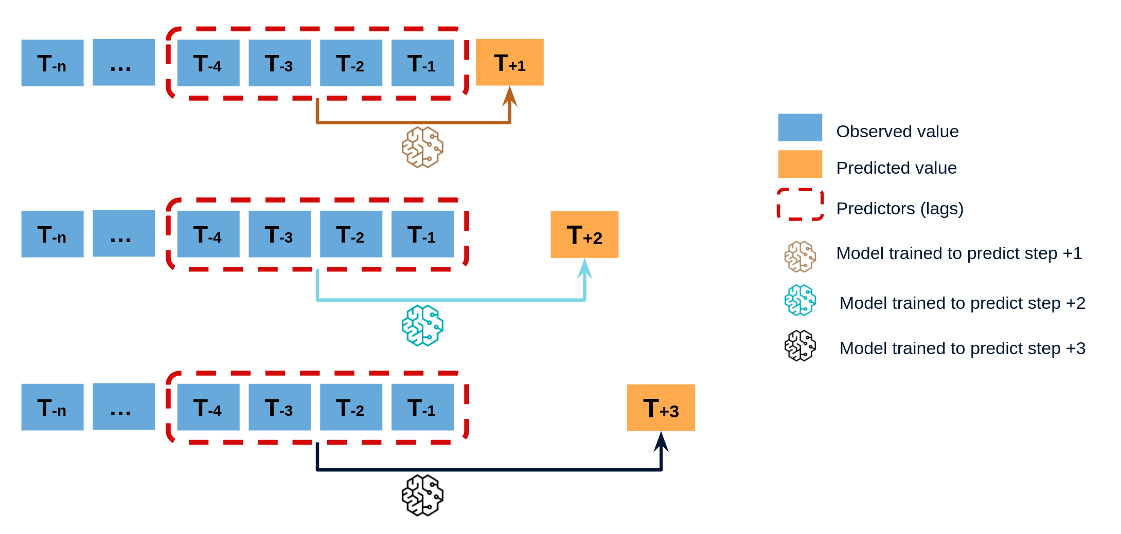
Direct multi-step forecasting is a time series forecasting strategy in which a separate model is trained to predict each step in the forecast horizon. This is in contrast to recursive multi-step forecasting, where a single model is used to make predictions for all future time steps by recursively using its own output as input.

Direct multi-step forecasting can be more computationally expensive than recursive forecasting since it requires training multiple models. However, it can often achieve better accuracy in certain scenarios, particularly when there are complex patterns and dependencies in the data that are difficult to capture with a single model.

This approach can be performed using the ForecasterDirect class, which can also incorporate one or multiple exogenous variables to improve the accuracy of the forecasts.

Diagram of direct multi-step forecasting.

Direct forecasting

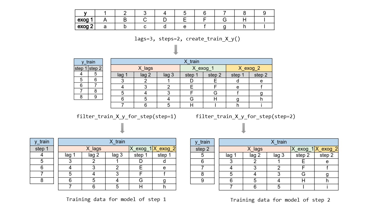
To train a ForecasterDirect a different training matrix is created for each model.

Transformation of a time series into matrices to train a direct multi-step forecasting model.

Libraries and data¶

In [1]:

# Libraries
# ==============================================================================
import pandas as pd
import matplotlib.pyplot as plt
from sklearn.linear_model import Ridge
from sklearn.metrics import mean_squared_error

from skforecast.datasets import fetch_dataset
from skforecast.preprocessing import RollingFeatures
from skforecast.direct import ForecasterDirect

# Libraries # ============================================================================== import pandas as pd import matplotlib.pyplot as plt from sklearn.linear_model import Ridge from sklearn.metrics import mean_squared_error from skforecast.datasets import fetch_dataset from skforecast.preprocessing import RollingFeatures from skforecast.direct import ForecasterDirect

In [2]:

# Download data
# ==============================================================================
data = fetch_dataset(
    name="h2o", raw=True, kwargs_read_csv={"names": ["y", "datetime"], "header": 0}
)

# Data preprocessing
# ==============================================================================
data['datetime'] = pd.to_datetime(data['datetime'], format='%Y-%m-%d')
data = data.set_index('datetime')
data = data.asfreq('MS')
data = data['y']
data = data.sort_index()

# Split train-test
# ==============================================================================
steps = 36
data_train = data[:-steps]
data_test  = data[-steps:]

# Plot
# ==============================================================================
fig, ax = plt.subplots(figsize=(6, 3))
data_train.plot(ax=ax, label='train')
data_test.plot(ax=ax, label='test')
ax.legend();

# Download data # ============================================================================== data = fetch_dataset( name="h2o", raw=True, kwargs_read_csv={"names": ["y", "datetime"], "header": 0} ) # Data preprocessing # ============================================================================== data['datetime'] = pd.to_datetime(data['datetime'], format='%Y-%m-%d') data = data.set_index('datetime') data = data.asfreq('MS') data = data['y'] data = data.sort_index() # Split train-test # ============================================================================== steps = 36 data_train = data[:-steps] data_test = data[-steps:] # Plot # ============================================================================== fig, ax = plt.subplots(figsize=(6, 3)) data_train.plot(ax=ax, label='train') data_test.plot(ax=ax, label='test') ax.legend();

h2o
---
Monthly expenditure ($AUD) on corticosteroid drugs that the Australian health
system had between 1991 and 2008.
Hyndman R (2023). fpp3: Data for Forecasting: Principles and Practice(3rd
Edition). http://pkg.robjhyndman.com/fpp3package/,https://github.com/robjhyndman
/fpp3package, http://OTexts.com/fpp3.
Shape of the dataset: (204, 2)

Create and train forecaster¶

✎ Note

ForecasterDirect includes the n_jobs parameter, allowing multi-process parallelization. This allows to train regressors for all steps simultaneously.

The benefits of parallelization depend on several factors, including the regressor used, the number of fits to be performed, and the volume of data involved. When the n_jobs parameter is set to 'auto', the level of parallelization is automatically selected based on heuristic rules that aim to choose the best option for each scenario.

For a more detailed look at parallelization, visit Parallelization in skforecast.

In [3]:

# Create and fit forecaster
# ==============================================================================
forecaster = ForecasterDirect(
                 regressor       = Ridge(),
                 steps           = 36,
                 lags            = 15,
                 window_features = RollingFeatures(stats=['mean'], window_sizes=10),
                 transformer_y   = None,
                 n_jobs          = 'auto'
             )

forecaster.fit(y=data_train)
forecaster

# Create and fit forecaster # ============================================================================== forecaster = ForecasterDirect( regressor = Ridge(), steps = 36, lags = 15, window_features = RollingFeatures(stats=['mean'], window_sizes=10), transformer_y = None, n_jobs = 'auto' ) forecaster.fit(y=data_train) forecaster

Out[3]:

ForecasterDirect

General Information

• Regressor: Ridge
• Lags: [ 1 2 3 4 5 6 7 8 9 10 11 12 13 14 15]
• Window features: ['roll_mean_10']
• Window size: 15
• Maximum steps to predict: 36
• Exogenous included: False
• Weight function included: False
• Differentiation order: None
• Creation date: 2024-11-08 16:36:08
• Last fit date: 2024-11-08 16:36:08
• Skforecast version: 0.14.0
• Python version: 3.11.10
• Forecaster id: None

Exogenous Variables

None

Data Transformations

• Transformer for y: None
• Transformer for exog: None

Training Information

• Training range: [Timestamp('1991-07-01 00:00:00'), Timestamp('2005-06-01 00:00:00')]
• Training index type: DatetimeIndex
• Training index frequency: MS

Regressor Parameters

{'alpha': 1.0, 'copy_X': True, 'fit_intercept': True, 'max_iter': None, 'positive': False, 'random_state': None, 'solver': 'auto', 'tol': 0.0001}

Fit Kwargs

{}

🛈 API Reference    🗎 User Guide

Prediction¶

When predicting, the value of steps must be less than or equal to the value of steps defined when initializing the forecaster. Starts at 1.

• If int only steps within the range of 1 to int are predicted.

• If list of int. Only the steps contained in the list are predicted.

• If None as many steps are predicted as were defined at initialization.

In [4]:

# Predict
# ==============================================================================
# Predict only a subset of steps
predictions = forecaster.predict(steps=[1, 5])
display(predictions)

# Predict # ============================================================================== # Predict only a subset of steps predictions = forecaster.predict(steps=[1, 5]) display(predictions)

2005-07-01    0.952188
2005-11-01    1.180630
Name: pred, dtype: float64

In [5]:

# Predict all steps defined in the initialization.
predictions = forecaster.predict()
display(predictions.head(3))

# Predict all steps defined in the initialization. predictions = forecaster.predict() display(predictions.head(3))

2005-07-01    0.952188
2005-08-01    1.004327
2005-09-01    1.115190
Freq: MS, Name: pred, dtype: float64

In [6]:

# Plot predictions
# ==============================================================================
fig, ax = plt.subplots(figsize=(6, 3))
data_train.plot(ax=ax, label='train')
data_test.plot(ax=ax, label='test')
predictions.plot(ax=ax, label='predictions')
ax.legend();

# Plot predictions # ============================================================================== fig, ax = plt.subplots(figsize=(6, 3)) data_train.plot(ax=ax, label='train') data_test.plot(ax=ax, label='test') predictions.plot(ax=ax, label='predictions') ax.legend();

In [7]:

# Prediction error
# ==============================================================================
predictions = forecaster.predict(steps=36)

error_mse = mean_squared_error(
                y_true = data_test,
                y_pred = predictions
            )
            
print(f"Test error (mse): {error_mse}")

# Prediction error # ============================================================================== predictions = forecaster.predict(steps=36) error_mse = mean_squared_error( y_true = data_test, y_pred = predictions ) print(f"Test error (mse): {error_mse}")

Test error (mse): 0.008447518677148016

Feature importances¶

Since ForecasterDirect fits one model per step, it is necessary to specify from which model retrieves its feature importances.

In [8]:

forecaster.get_feature_importances(step=1)

forecaster.get_feature_importances(step=1)

Out[8]:

	feature	importance
11	lag_12	0.551517
10	lag_11	0.153757
0	lag_1	0.138408
12	lag_13	0.056914
1	lag_2	0.050145
2	lag_3	0.043166
9	lag_10	0.019264
15	roll_mean_10	0.016897
8	lag_9	0.010420
7	lag_8	-0.014137
5	lag_6	-0.014835
4	lag_5	-0.019494
3	lag_4	-0.021308
6	lag_7	-0.022662
14	lag_15	-0.035939
13	lag_14	-0.071710

Training and prediction matrices¶

While the primary goal of building forecasting models is to predict future values, it is equally important to evaluate if the model is effectively learning from the training data. Analyzing predictions on the training data or exploring the prediction matrices is crucial for assessing model performance and understanding areas for optimization. This process can help identify issues like overfitting or underfitting, as well as provide deeper insights into the model’s decision-making process. Check the How to Extract Training and Prediction Matrices user guide for more information.