Recursive multi-step forecasting¶

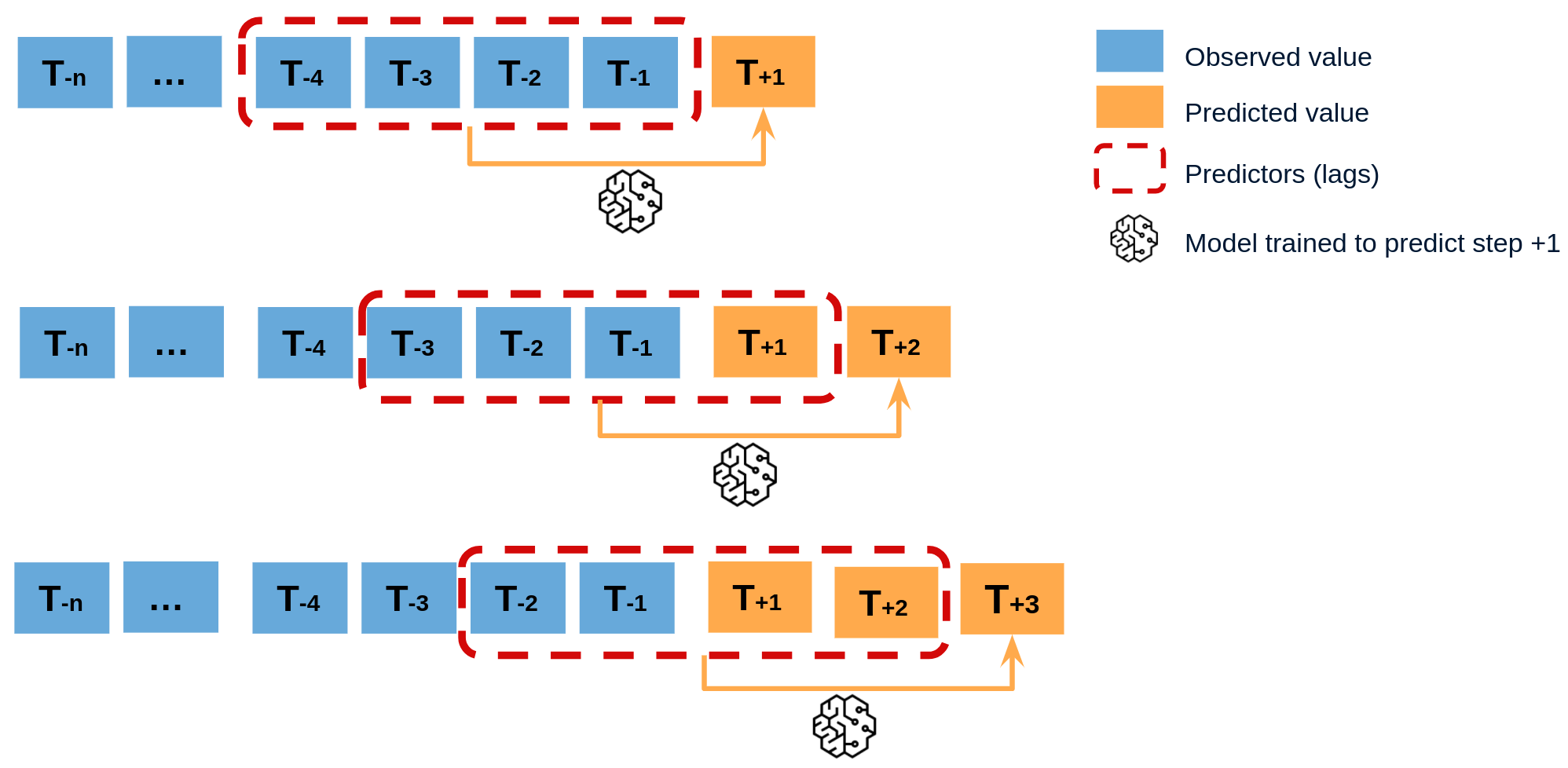
Recursive multi-step forecasting involves using the predicted values from previous time steps as input to forecast the values for the subsequent time steps. The model initially predicts one time step ahead and then uses that forecast as an input for the next time step, continuing this recursive process until the desired forecast horizon is reached.

To clarify, since the value of $t_{n-1}$ is required to predict $t_{n}$, and $t_{n-1}$ is unknown, a recursive process is applied in which, each new prediction is based on the previous one.

Diagram of recursive multi-step forecasting

Recursive forecasting

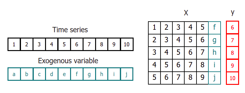
When using machine learning models for recursive multi-step forecasting, one of the major challenges is transforming the time series data into a matrix format that relates each value of the series to the preceding time window (lags). This process can be complex and time-consuming, requiring careful feature engineering to ensure the model can accurately capture the underlying patterns in the data.

Time series transformation including an exogenous variable

By using the classes ForecasterRecursive, it is possible to build machine learning models for recursive multi-step forecasting with ease. These classes can automatically transform the time series data into a matrix format suitable for input to a machine learning algorithm, and provide a range of options for tuning the model parameters to achieve the best possible performance.

Libraries and data¶

In [ ]:

# Libraries
# ==============================================================================
import pandas as pd
import matplotlib.pyplot as plt
from lightgbm import LGBMRegressor
from sklearn.metrics import mean_squared_error

from skforecast.datasets import fetch_dataset
from skforecast.preprocessing import RollingFeatures
from skforecast.recursive import ForecasterRecursive

# Libraries # ============================================================================== import pandas as pd import matplotlib.pyplot as plt from lightgbm import LGBMRegressor from sklearn.metrics import mean_squared_error from skforecast.datasets import fetch_dataset from skforecast.preprocessing import RollingFeatures from skforecast.recursive import ForecasterRecursive

In [2]:

# Download data
# ==============================================================================
data = fetch_dataset(
    name="h2o", raw=True, kwargs_read_csv={"names": ["y", "datetime"], "header": 0}
)

# Data preprocessing
# ==============================================================================
data['datetime'] = pd.to_datetime(data['datetime'], format='%Y-%m-%d')
data = data.set_index('datetime')
data = data.asfreq('MS')
data = data['y']
data = data.sort_index()

# Split train-test
# ==============================================================================
steps = 36
data_train = data[:-steps]
data_test  = data[-steps:]

# Plot
# ==============================================================================
fig, ax = plt.subplots(figsize=(6, 3))
data_train.plot(ax=ax, label='train')
data_test.plot(ax=ax, label='test')
ax.legend();

# Download data # ============================================================================== data = fetch_dataset( name="h2o", raw=True, kwargs_read_csv={"names": ["y", "datetime"], "header": 0} ) # Data preprocessing # ============================================================================== data['datetime'] = pd.to_datetime(data['datetime'], format='%Y-%m-%d') data = data.set_index('datetime') data = data.asfreq('MS') data = data['y'] data = data.sort_index() # Split train-test # ============================================================================== steps = 36 data_train = data[:-steps] data_test = data[-steps:] # Plot # ============================================================================== fig, ax = plt.subplots(figsize=(6, 3)) data_train.plot(ax=ax, label='train') data_test.plot(ax=ax, label='test') ax.legend();

h2o
---
Monthly expenditure ($AUD) on corticosteroid drugs that the Australian health
system had between 1991 and 2008.
Hyndman R (2023). fpp3: Data for Forecasting: Principles and Practice(3rd
Edition). http://pkg.robjhyndman.com/fpp3package/,https://github.com/robjhyndman
/fpp3package, http://OTexts.com/fpp3.
Shape of the dataset: (204, 2)

Create and train forecaster¶

In [3]:

# Create and fit forecaster
# ==============================================================================
forecaster = ForecasterRecursive(
                 regressor       = LGBMRegressor(random_state=123, verbose=-1),
                 lags            = 15,
                 window_features = RollingFeatures(stats=['mean'], window_sizes=10)
             )

forecaster.fit(y=data_train)
forecaster

# Create and fit forecaster # ============================================================================== forecaster = ForecasterRecursive( regressor = LGBMRegressor(random_state=123, verbose=-1), lags = 15, window_features = RollingFeatures(stats=['mean'], window_sizes=10) ) forecaster.fit(y=data_train) forecaster

Out[3]:

ForecasterRecursive

General Information

• Regressor: LGBMRegressor
• Lags: [ 1 2 3 4 5 6 7 8 9 10 11 12 13 14 15]
• Window features: ['roll_mean_10']
• Window size: 15
• Exogenous included: False
• Weight function included: False
• Differentiation order: None
• Creation date: 2024-11-08 16:33:48
• Last fit date: 2024-11-08 16:33:48
• Skforecast version: 0.14.0
• Python version: 3.11.10
• Forecaster id: None

Exogenous Variables

None

Data Transformations

• Transformer for y: None
• Transformer for exog: None

Training Information

• Training range: [Timestamp('1991-07-01 00:00:00'), Timestamp('2005-06-01 00:00:00')]
• Training index type: DatetimeIndex
• Training index frequency: MS

Regressor Parameters

{'boosting_type': 'gbdt', 'class_weight': None, 'colsample_bytree': 1.0, 'importance_type': 'split', 'learning_rate': 0.1, 'max_depth': -1, 'min_child_samples': 20, 'min_child_weight': 0.001, 'min_split_gain': 0.0, 'n_estimators': 100, 'n_jobs': None, 'num_leaves': 31, 'objective': None, 'random_state': 123, 'reg_alpha': 0.0, 'reg_lambda': 0.0, 'subsample': 1.0, 'subsample_for_bin': 200000, 'subsample_freq': 0, 'verbose': -1}

Fit Kwargs

{}

🛈 API Reference    🗎 User Guide

Prediction¶

In [4]:

# Predict
# ==============================================================================
predictions = forecaster.predict(steps=36)
predictions.head(3)

# Predict # ============================================================================== predictions = forecaster.predict(steps=36) predictions.head(3)

Out[4]:

2005-07-01    1.026507
2005-08-01    1.042429
2005-09-01    1.116730
Freq: MS, Name: pred, dtype: float64

In [5]:

# Plot predictions
# ==============================================================================
fig, ax = plt.subplots(figsize=(6, 3))
data_train.plot(ax=ax, label='train')
data_test.plot(ax=ax, label='test')
predictions.plot(ax=ax, label='predictions')
ax.legend();

# Plot predictions # ============================================================================== fig, ax = plt.subplots(figsize=(6, 3)) data_train.plot(ax=ax, label='train') data_test.plot(ax=ax, label='test') predictions.plot(ax=ax, label='predictions') ax.legend();

In [6]:

# Prediction error
# ==============================================================================
error_mse = mean_squared_error(
                y_true = data_test,
                y_pred = predictions
            )
print(f"Test error (mse): {error_mse}")

# Prediction error # ============================================================================== error_mse = mean_squared_error( y_true = data_test, y_pred = predictions ) print(f"Test error (mse): {error_mse}")

Test error (mse): 0.006632513357651682

Prediction intervals¶

A prediction interval defines the interval within which the true value of y is expected to be found with a given probability. For example, the prediction interval (1, 99) can be expected to contain the true prediction value with 98% probability.

By default, every forecaster can estimate prediction intervals using the method predict_interval. For a detailed explanation of the different prediction intervals available in skforecast visit Probabilistic forecasting.

In [7]:

# Predict intervals
# ==============================================================================
predictions = forecaster.predict_interval(steps=36, interval=[5, 95], n_boot=100)
predictions.head(3)

# Predict intervals # ============================================================================== predictions = forecaster.predict_interval(steps=36, interval=[5, 95], n_boot=100) predictions.head(3)

Out[7]:

	pred	lower_bound	upper_bound
2005-07-01	1.026507	0.986691	1.063817
2005-08-01	1.042429	1.001314	1.100771
2005-09-01	1.116730	1.079703	1.153881

In [8]:

# Plot prediction interval
# ==============================================================================
fig, ax = plt.subplots(figsize=(6, 3))
data_test.plot(ax=ax, label="test")
predictions['pred'].plot(ax=ax, label="prediction")
ax.fill_between(
    predictions.index,
    predictions['lower_bound'],
    predictions['upper_bound'],
    color = 'blue',
    alpha = 0.3,
    label = '80% interval'
)
ax.legend(loc="upper left");

# Plot prediction interval # ============================================================================== fig, ax = plt.subplots(figsize=(6, 3)) data_test.plot(ax=ax, label="test") predictions['pred'].plot(ax=ax, label="prediction") ax.fill_between( predictions.index, predictions['lower_bound'], predictions['upper_bound'], color = 'blue', alpha = 0.3, label = '80% interval' ) ax.legend(loc="upper left");

Feature importances¶

In [9]:

forecaster.get_feature_importances()

forecaster.get_feature_importances()

Out[9]:

	feature	importance
11	lag_12	88
10	lag_11	47
1	lag_2	45
0	lag_1	35
12	lag_13	35
15	roll_mean_10	30
8	lag_9	29
6	lag_7	28
5	lag_6	26
13	lag_14	24
2	lag_3	23
14	lag_15	20
4	lag_5	19
9	lag_10	19
3	lag_4	17
7	lag_8	15

Training and prediction matrices¶

While the primary goal of building forecasting models is to predict future values, it is equally important to evaluate if the model is effectively learning from the training data. Analyzing predictions on the training data or exploring the prediction matrices is crucial for assessing model performance and understanding areas for optimization. This process can help identify issues like overfitting or underfitting, as well as provide deeper insights into the model’s decision-making process. Check the How to Extract Training and Prediction Matrices user guide for more information.

Differentiation¶

Time series differentiation involves computing the differences between consecutive observations in the time series. When it comes to training forecasting models, differentiation offers the advantage of focusing on relative rates of change rather than directly attempting to model the absolute values. Once the predictions have been estimated, this transformation can be easily reversed to restore the values to their original scale.

💡 Tip

To learn more about modeling time series differentiation, visit our example: Modelling time series trend with tree based models.

In [10]:

# Create and fit forecaster
# ==============================================================================
forecaster = ForecasterRecursive(
                 regressor       = LGBMRegressor(random_state=123, verbose=-1),
                 lags            = 15,
                 differentiation = 1
             )

forecaster.fit(y=data_train)
forecaster

# Create and fit forecaster # ============================================================================== forecaster = ForecasterRecursive( regressor = LGBMRegressor(random_state=123, verbose=-1), lags = 15, differentiation = 1 ) forecaster.fit(y=data_train) forecaster

Out[10]:

ForecasterRecursive

General Information

• Regressor: LGBMRegressor
• Lags: [ 1 2 3 4 5 6 7 8 9 10 11 12 13 14 15]
• Window features: None
• Window size: 16
• Exogenous included: False
• Weight function included: False
• Differentiation order: 1
• Creation date: 2024-11-08 16:33:51
• Last fit date: 2024-11-08 16:33:51
• Skforecast version: 0.14.0
• Python version: 3.11.10
• Forecaster id: None

Exogenous Variables

None

Data Transformations

• Transformer for y: None
• Transformer for exog: None

Training Information

• Training range: [Timestamp('1991-07-01 00:00:00'), Timestamp('2005-06-01 00:00:00')]
• Training index type: DatetimeIndex
• Training index frequency: MS

Regressor Parameters

{'boosting_type': 'gbdt', 'class_weight': None, 'colsample_bytree': 1.0, 'importance_type': 'split', 'learning_rate': 0.1, 'max_depth': -1, 'min_child_samples': 20, 'min_child_weight': 0.001, 'min_split_gain': 0.0, 'n_estimators': 100, 'n_jobs': None, 'num_leaves': 31, 'objective': None, 'random_state': 123, 'reg_alpha': 0.0, 'reg_lambda': 0.0, 'subsample': 1.0, 'subsample_for_bin': 200000, 'subsample_freq': 0, 'verbose': -1}

Fit Kwargs

{}

🛈 API Reference    🗎 User Guide

In [11]:

# Predict
# ==============================================================================
predictions = forecaster.predict(steps=36)
predictions.head(3)

# Predict # ============================================================================== predictions = forecaster.predict(steps=36) predictions.head(3)

Out[11]:

2005-07-01    0.909529
2005-08-01    0.941633
2005-09-01    1.007650
Freq: MS, Name: pred, dtype: float64