Forecasting with foundation models
Foundation models (FMs) have triggered a fundamental paradigm shift in time series forecasting, moving the field away from modelling for each dataset and towards generalised representation learning. Driven by the same architectural breakthroughs that power Large Language Models (LLMs), FMs bring zero-shot and in-context learning capabilities to temporal data.
In the context of forecasting, a foundation model is a massively scaled neural network (typically Transformer-based) that has been pre-trained on highly diverse, cross-domain datasets spanning finance, weather, web traffic, retail and more.
Models such as Amazon Chronos, Google TimesFM 2.5, Salesforce Moirai-2, Soda-INRIA TabICL, Prior Labs' TabPFN-TS, and The Forecasting Company T0 treat forecasting as a foundation-model problem. Many frame it as sequence modelling, processing temporal data either as quantized discrete tokens (as in Chronos, which applies scalar quantization) or as continuous patch embeddings (as in TimesFM and Moirai, which group consecutive time steps into fixed-length patches before encoding them); others (TabICL, TabPFN-TS) recast it as tabular in-context learning. Having internalised the structural priors of millions of series during pre-training, they can infer trends, seasonality, and complex dynamics in unseen data without any task-specific weight updates.
Foundation Models vs. Machine Learning Models
Foundation models and traditional machine learning models approach forecasting in fundamentally different ways. Understanding these distinctions is crucial for knowing when and how to deploy each method.
Zero-Shot Prediction
Machine learning models require a training phase. You must fit the model on your historical target data so the algorithm can learn the optimal weights and parameters for your specific time series. Foundation models, however, are capable of zero-shot inference. Because their highly generalized weights are already frozen from the massive pre-training phase, they can generate accurate forecasts on your data immediately, leveraging their pre-existing latent representations rather than learning your dataset from scratch.
The Role of the fit Method
Machine learning models must be trained: calling .fit() optimizes the model's internal parameters by minimizing a loss function on your historical data. Foundation models, by contrast, arrive pre-trained: their weights are fixed and are never updated. Calling .fit() on a foundation model is not a training step; it simply stores the historical context (observations, frequency, and any scaling factors) needed at inference time. In some implementations, calling .fit() is entirely optional before prediction.
Context Window vs. Engineered Lags
Machine learning models rely on explicitly engineered features; they require creating a tabular dataset where past values are used as columns to predict the target. Foundation models rely on a context window. You pass a raw, sequential chunk of recent historical data (e.g., the last 512 observations) directly into the model at inference time. The attention mechanism inside the model automatically decides which past data points are most relevant.
In summary, foundation models represent a fundamental paradigm shift, replacing the traditional train → predict pipeline with a pre-train → (context + predict) approach. As major research institutions with access to millions of diverse time series carry out the computationally intensive pre-training phase, end users are completely freed from model training.
However, there is no such thing as a free lunch in machine learning. Skipping the training phase results in a heavier burden during the inference phase. Because their weights are frozen, these models cannot adapt to your data through training. Instead, they adapt implicitly at inference time by processing the historical context through their attention mechanism. Each prediction therefore requires ingesting and attending over a large sequence of raw observations in real time. Consequently, the main drawback of zero-shot forecasting is that the inference process is significantly slower, more computationally expensive and requires your data pipeline to continuously provide large amounts of historical context at runtime.
| - | ML Model | Foundation Model |
|---|---|---|
| fit | Trains model, updates weights | Stores context & metadata |
| predict | Uses learned weights | Processes context via attention |
| Data required at train time | Full history | Not required |
| Data required at predict time | Last lags observations | Full context window |
| Computational cost | At train time | At inference time |
Impact of the context length
Because foundation forecasting models are highly generalized, they lack intrinsic knowledge of your specific dataset. To compensate, they rely on a context window, a specific period of recent historical data, to adapt to your unique scenario at inference time. This context acts as the model's short-term memory, allowing it to calculate the current trajectory of your data and identify whether the series is trending upward, accelerating, or flattening out.
The length of this context window is critical for capturing seasonality and recurring events. To accurately predict a pattern, such as a weekly sales spike or a yearly cycle, the model must actually observe that pattern within the provided history. For instance, if your data has a 365-day seasonality, providing 400 days of context allows the model to recognize and project the cycle, whereas a 30-day window would cause the model to miss the pattern entirely, resulting in a flat or inaccurate forecast.
However, increasing the context length to improve accuracy introduces a significant computational trade-off. Because most foundation models are built on Transformer architectures, the computational complexity of their attention mechanism often scales quadratically (
Ultimately, effectively utilizing foundation models requires carefully evaluating this trade-off. The best practice is to analyze the context size and select the shortest possible window that still achieves high predictive performance. Striking this balance ensures accurate, pattern-aware forecasts while preventing the unnecessary waste of computational resources.
Comparative charts of prediction error and elapsed time based on context length.
✏️ Note
For more details about foundation models, visit Forecasting: Principles and Practice, the Pythonic Way.
Foundation Models in skforecast
Skforecast's integration is built on two layers. First, FoundationModel acts as a unified wrapper that adapts each model's native API (Chronos-2, TimesFM 2.5, Moirai-2, TabICL, TabPFN-TS, TFC T0) behind a familiar scikit-learn interface (fit, predict, get_params). Second, ForecasterFoundation wraps that estimator to unlock the full skforecast ecosystem. It exposes the same interface as any other skforecast forecaster, meaning users can use backtesting, prediction intervals, and multi-series support with the exact same code.
Supported Foundation Models
| Chronos | TimesFM | Moirai | TabICL | TabPFN-TS | T0 | |
|---|---|---|---|---|---|---|
| Provider | Amazon | Salesforce | Soda-Inria | Prior Labs | The Forecasting Company | |
| GitHub | chronos-forecasting | timesfm | uni2ts | tabicl | tabpfn-time-series | tfc-t0 |
| Documentation | Chronos models | TimesFM models | Moirai-R models | TabICL Docs | Prior Labs Docs | t0-alpha model card |
| Available model IDs | amazon/chronos-2 autogluon/chronos-2-small autogluon/chronos-2-synth |
google/timesfm-2.5-200m-pytorch | Salesforce/moirai-2.0-R-small | soda-inria/tabicl | priorlabs/tabpfn-ts | theforecastingcompany/t0-alpha |
| Backend | PyTorch | PyTorch | PyTorch | PyTorch | PyTorch | PyTorch |
| Forecasting type | Zero-shot | Zero-shot | Zero-shot | Zero-shot | Zero-shot | Zero-shot |
| Default context_length | 8192 | 512 | 2048 | 4096 | 32768 | 8192 |
| Max context_length | 8192 | 16384 | 2048 | 4096 | No hard limit (practical memory ceiling ~65536) | No hard limit, set via context_length |
| max_horizon | No hard limit, set via steps at predict time |
512 | No hard limit, set via steps at predict time |
No hard limit, set via steps at predict time |
No hard limit, set via steps at predict time |
No hard limit, set via steps at predict time |
| Point forecast | Median (0.5 quantile) | Mean (dedicated output array) | Median (0.5 quantile) | Mean (default, configurable to median) | Median (default, configurable to mean/mode) | Median (0.5 quantile) |
| Covariate support (exog) | Yes | No | No | Yes | Yes | Yes |
| cross_learning parameter | Yes (multi-series mode only) | No | No | No | No | No |
| Install command | pip install chronos-forecasting |
pip install git+https://github.com/google-research/timesfm.git |
pip install uni2ts |
pip install tabicl[forecast] |
pip install tabpfn-time-series |
pip install tfc-t0 |
💡 Tip
All models run on the CPU. However, a CUDA GPU is recommended for faster inference, especially with long context windows. The MPS backend is also detected automatically by PyTorch and can benefit Apple Silicon users.
It is important to note that context length significantly impacts inference speed. Larger contexts provide the models with more information, but they increase processing time. Although these models boast massive context capacities, shorter contexts often achieve similar results much faster for most use cases.
Input Data Formats
ForecasterFoundation accepts several data formats for both the target series and exogenous variables.
Target Series (series)
The series parameter in the .fit() method supports both single-series and multi-series (global model) configurations.
| Mode | Allowed Data Type | Description |
|---|---|---|
| Single-Series | pd.Series |
A single time series with a named index. |
| Multi-Series (Wide) | pd.DataFrame |
Each column represents a separate time series. |
| Multi-Series (Long) | pd.DataFrame |
MultiIndex (Level 0: series ID, Level 1: DatetimeIndex). |
| Multi-Series (Dict) | dict[str, pd.Series] |
Keys are series identifiers, values are pandas Series. |
💡 Tip
While Long-format DataFrames are supported, they are converted to dictionaries internally. For best performance, pass a dict[str, pd.Series] directly.
Exogenous Variables (exog)
Exogenous variables must be aligned with the target series index. Currently, Chronos, TabICL, TabPFN-TS, and TFC-T0 support covariates (see the Supported Foundation Models table). TimesFM and Moirai do not accept exogenous variables.
| Mode | Allowed Data Type | Description |
|---|---|---|
| Single-Series | pd.Series or pd.DataFrame |
Aligned to the target series index. |
| Multi-Series (Dict) | dict[str, pd.Series \| pd.DataFrame \| None] |
One entry per series. |
| Multi-Series (Broadcast) | pd.Series or pd.DataFrame |
Automatically applied to all series. |
| Multi-Series (Long) | pd.DataFrame |
MultiIndex (Level 0: series ID, Level 1: DatetimeIndex). |
Libraries and data
# Libraries
# ==============================================================================
import os
import pandas as pd
import torch
import time
import matplotlib.pyplot as plt
from skforecast.datasets import fetch_dataset
from skforecast.foundation import FoundationModel, ForecasterFoundation
from skforecast.model_selection import (
    TimeSeriesFold,
    backtesting_foundation
)
from skforecast.plot import set_dark_theme

color = '\033[1m\033[38;5;208m'
print(f"{color}torch version: {torch.__version__}")
print(f"  Cuda available : {torch.cuda.is_available()}")
print(f"  MPS available  : {torch.backends.mps.is_available()}")
torch version: 2.12.1+cpu
  Cuda available : False
  MPS available  : False
# Data download
# ==============================================================================
data = fetch_dataset(name='vic_electricity')

# Aggregating in 1H intervals
# ==============================================================================
# The Date column is eliminated so that it does not generate an error when aggregating.
data = data.drop(columns="Date")
data = (
    data
    .resample(rule="h", closed="left", label="right")
    .agg({
        "Demand": "mean",
        "Temperature": "mean",
        "Holiday": "mean",
    })
)
data.head(3)
╭──────────────────────────── vic_electricity ─────────────────────────────╮
│ Description:                                                             │
│ Half-hourly electricity demand for Victoria, Australia                   │
│                                                                          │
│ Source:                                                                  │
│ O'Hara-Wild M, Hyndman R, Wang E, Godahewa R (2022).tsibbledata: Diverse │
│ Datasets for 'tsibble'. https://tsibbledata.tidyverts.org/,              │
│ https://github.com/tidyverts/tsibbledata/.                               │
│ https://tsibbledata.tidyverts.org/reference/vic_elec.html                │
│                                                                          │
│ URL:                                                                     │
│ https://raw.githubusercontent.com/skforecast/skforecast-                 │
│ datasets/main/data/vic_electricity.csv                                   │
│                                                                          │
│ Shape: 52608 rows x 4 columns                                            │
╰──────────────────────────────────────────────────────────────────────────╯
| Demand | Temperature | Holiday | |
|---|---|---|---|
| Time | |||
| 2011-12-31 14:00:00 | 4323.095350 | 21.225 | 1.0 |
| 2011-12-31 15:00:00 | 3963.264688 | 20.625 | 1.0 |
| 2011-12-31 16:00:00 | 3950.913495 | 20.325 | 1.0 |
# Split data into train-test
# ==============================================================================
data = data.loc['2012-01-01 00:00:00':'2014-12-30 23:00:00', :].copy()
end_train = '2014-11-30 23:59:00'
data_train = data.loc[: end_train, :].copy()
data_test  = data.loc[end_train:, :].copy()

print(f"Train dates: {data_train.index.min()} --- {data_train.index.max()}  (n={len(data_train)})")
print(f"Test dates : {data_test.index.min()} --- {data_test.index.max()}  (n={len(data_test)})")
Train dates: 2012-01-01 00:00:00 --- 2014-11-30 23:00:00  (n=25560)
Test dates : 2014-12-01 00:00:00 --- 2014-12-30 23:00:00  (n=720)
Chronos
A ForecasterFoundation is created using Amazon's Chronos-2-small model.
# Create ForecasterFoundation
# ==============================================================================
estimator = FoundationModel(model_id="autogluon/chronos-2-small", context_length=500)
forecaster = ForecasterFoundation(estimator=estimator)
Each adapter accepts additional keyword arguments that control model-specific behavior (e.g., context_length, device_map, torch_dtype). These can be passed directly through the FoundationModel constructor.
For the full list of available parameters, see the API reference: ChronosAdapter, TimesFMAdapter, MoiraiAdapter, TabICLAdapter.
💡 Tip
While .fit() is used here to store the historical context and metadata, it is not strictly required. Foundation models can generate forecasts by passing the context directly to .predict() via the context parameter. However, calling .fit() first simplifies subsequent calls to .predict(), .predict_interval(), and .predict_quantiles().
# Train ForecasterFoundation
# ==============================================================================
forecaster.fit(
    series = data_train["Demand"],
    exog   = data_train[["Temperature", "Holiday"]]
)
forecaster
ForecasterFoundation
General Information
- Model ID: autogluon/chronos-2-small
- Context length: 500
- Window size: 500
- Series names: Demand
- Exogenous included: True
- Creation date: 2026-06-18 12:13:00
- Last fit date: 2026-06-18 12:13:00
- Skforecast version: 0.23.0
- Python version: 3.12.13
- Forecaster id: None
Exogenous Variables
Temperature, Holiday
Training Information
- Context range: 'Demand': ['2012-01-01 00:00:00', '2014-11-30 23:00:00']
- Training index type: DatetimeIndex
- Training index frequency:
Model Parameters
- cross_learning: False
- context_length: 500
- device_map: auto
- torch_dtype: None
- predict_kwargs: None
Three methods can be used to predict the next predict(), predict_interval(), and predict_quantiles(). All these methods allow for passing context and context_exog to override the historical context used by the underlying model to generate predictions.
# Predictions: point forecast
# ==============================================================================
steps = 24
predictions = forecaster.predict(
                  steps = steps,
                  exog  = data_test[["Temperature", "Holiday"]]
              )

predictions.head(3)
| level | pred | |
|---|---|---|
| 2014-12-01 00:00:00 | Demand | 5527.679199 |
| 2014-12-01 01:00:00 | Demand | 5511.500977 |
| 2014-12-01 02:00:00 | Demand | 5457.792480 |
# Predictions: intervals
# ==============================================================================
predictions_intervals = forecaster.predict_interval(
                            steps    = steps,
                            exog     = data_test[["Temperature", "Holiday"]],
                            interval = [0.1, 0.9],  # 80% prediction interval
                        )

predictions_intervals.head(3)
| level | pred | lower_bound | upper_bound | |
|---|---|---|---|---|
| 2014-12-01 00:00:00 | Demand | 5527.679199 | 5372.815918 | 5689.794434 |
| 2014-12-01 01:00:00 | Demand | 5511.500977 | 5318.045898 | 5733.492188 |
| 2014-12-01 02:00:00 | Demand | 5457.792480 | 5241.040527 | 5717.425781 |
Backtesting
Backtesting with foundation models works differently than with traditional machine learning forecasters. Since the model's weights are frozen and never updated, the concept of refitting does not apply. The refit and fixed_train_size arguments in TimeSeriesFold are ignored internally.
Instead, what changes across folds is the context window. As backtesting progresses, the amount of historical data available grows. At each fold, the model receives the most recent observations up to the fold boundary. This process has two phases: first, the context expands as more historical data becomes available with each fold; once the available history exceeds the model's context_length, the context stops growing and instead slides forward, always using the last context_length observations before the fold boundary.
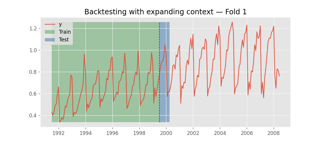
Backtesting with expanding context window.
To learn more about backtesting, visit the backtesting user guide.
# Backtesting
# ==============================================================================
cv = TimeSeriesFold(
         steps              = 24,
         initial_train_size = len(data.loc[:end_train]),
         refit              = False
     )

metrics_chronos, backtest_predictions = backtesting_foundation(
    forecaster        = forecaster,
    series            = data['Demand'],
    exog              = data[["Temperature", "Holiday"]],
    cv                = cv,
    metric            = 'mean_absolute_error',
    suppress_warnings = True
)

print("Backtest metrics")
display(metrics_chronos)
print("")
print("Backtest predictions")
backtest_predictions.head(4)
0%| | 0/30 [00:00<?, ?it/s]
Backtest metrics
| mean_absolute_error | |
|---|---|
| 0 | 171.266968 |
Backtest predictions
| level | fold | pred | |
|---|---|---|---|
| 2014-12-01 00:00:00 | Demand | 0 | 5527.679199 |
| 2014-12-01 01:00:00 | Demand | 0 | 5511.500977 |
| 2014-12-01 02:00:00 | Demand | 0 | 5457.792480 |
| 2014-12-01 03:00:00 | Demand | 0 | 5402.819824 |
# Plot predictions
# ==============================================================================
set_dark_theme()
fig, ax = plt.subplots(figsize=(7, 3))
data_test['Demand'].plot(ax=ax, label='test')
backtest_predictions['pred'].plot(ax=ax, label='predictions')
ax.legend();

Multiple series (global model)
The class ForecasterFoundation allows modeling and forecasting multiple series with a single model.
# Data
# ==============================================================================
data_multiseries = fetch_dataset(name="items_sales")
display(data_multiseries.head(3))
╭─────────────────────── items_sales ───────────────────────╮
│ Description:                                              │
│ Simulated time series for the sales of 3 different items. │
│                                                           │
│ Source:                                                   │
│ Simulated data.                                           │
│                                                           │
│ URL:                                                      │
│ https://raw.githubusercontent.com/skforecast/skforecast-  │
│ datasets/main/data/simulated_items_sales.csv              │
│                                                           │
│ Shape: 1097 rows x 3 columns                              │
╰───────────────────────────────────────────────────────────╯
| item_1 | item_2 | item_3 | |
|---|---|---|---|
| date | |||
| 2012-01-01 | 8.253175 | 21.047727 | 19.429739 |
| 2012-01-02 | 22.777826 | 26.578125 | 28.009863 |
| 2012-01-03 | 27.549099 | 31.751042 | 32.078922 |
# Split data into train-test
# ==============================================================================
end_train = '2014-07-15 23:59:00'
data_multiseries_train = data_multiseries.loc[:end_train, :].copy()
data_multiseries_test  = data_multiseries.loc[end_train:, :].copy()
# Plot time series
# ==============================================================================
set_dark_theme()
fig, axes = plt.subplots(nrows=3, ncols=1, figsize=(7, 5), sharex=True)

for i, col in enumerate(data_multiseries.columns):
    data_multiseries_train[col].plot(ax=axes[i], label='train')
    data_multiseries_test[col].plot(ax=axes[i], label='test')
    axes[i].set_title(col)
    axes[i].set_ylabel('sales')
    axes[i].set_xlabel('')
    axes[i].legend(loc='upper left')

fig.tight_layout()
plt.show();

In this example, instead of calling fit(), the context is passed directly to the predict() method.
# Create and train ForecasterFoundation
# ==============================================================================
estimator = FoundationModel(model_id = "autogluon/chronos-2-small", context_length=500)
forecaster = ForecasterFoundation(estimator = estimator)

# fit() is optional; context is passed directly to predict()
# forecaster.fit(series=data_multiseries_train)

forecaster
ForecasterFoundation
General Information
- Model ID: autogluon/chronos-2-small
- Context length: 500
- Window size: 500
- Series names: None
- Exogenous included: False
- Creation date: 2026-06-18 12:13:03
- Last fit date: None
- Skforecast version: 0.23.0
- Python version: 3.12.13
- Forecaster id: None
Exogenous Variables
None
Training Information
- Context range: Not fitted
- Training index type: Not fitted
- Training index frequency: Not fitted
Model Parameters
- cross_learning: False
- context_length: 500
- device_map: auto
- torch_dtype: None
- predict_kwargs: None
# Predictions for all series (levels)
# ==============================================================================
steps = len(data_multiseries_test)
predictions_items = forecaster.predict(
                        steps   = steps,
                        levels  = None,  # All levels are predicted
                        context = data_multiseries_train
                    )

predictions_items.head()
╭────────────────────────────────── InputTypeWarning ──────────────────────────────────╮
│ Passing a DataFrame (either wide or long format) as `series` requires additional     │
│ internal transformations, which can increase computational time. It is recommended   │
│ to use a dictionary of pandas Series instead. For more details, see:                 │
│ https://skforecast.org/latest/user_guides/independent-multi-time-series-forecasting. │
│ html#input-data                                                                      │
│                                                                                      │
│ Category : skforecast.exceptions.InputTypeWarning                                    │
│ Location :                                                                           │
│ /opt/homebrew/Caskroom/miniconda/base/envs/skforecast_py12/lib/python3.12/site-packa │
│ ges/skforecast/utils/utils.py:3072                                                   │
│ Suppress : warnings.simplefilter('ignore', category=InputTypeWarning)                │
╰──────────────────────────────────────────────────────────────────────────────────────╯
| level | pred | |
|---|---|---|
| 2014-07-16 | item_1 | 25.523060 |
| 2014-07-16 | item_2 | 10.456669 |
| 2014-07-16 | item_3 | 11.862239 |
| 2014-07-17 | item_1 | 25.296780 |
| 2014-07-17 | item_2 | 10.701235 |
# Plot predictions
# ==============================================================================
set_dark_theme()
fig, axes = plt.subplots(nrows=3, ncols=1, figsize=(7, 5), sharex=True)

for i, col in enumerate(data_multiseries.columns):

    data_multiseries_train[col].plot(ax=axes[i], label='train')
    data_multiseries_test[col].plot(ax=axes[i], label='test')
    predictions_items.query(f"level == '{col}'")['pred'].plot(
        ax=axes[i], label='predictions', color='white'
    )

    axes[i].set_title(col)
    axes[i].set_ylabel('sales')
    axes[i].set_xlabel('')
    axes[i].legend(loc='upper left')

fig.tight_layout()
plt.show();

# Interval predictions for item_1 and item_2
# ==============================================================================
predictions_intervals = forecaster.predict_interval(
                            steps    = 24,
                            levels   = ['item_1', 'item_2'],
                            context  = data_multiseries_train,
                            interval = [0.1, 0.9],  # 80% prediction interval
                        )

predictions_intervals.head()
╭────────────────────────────────── InputTypeWarning ──────────────────────────────────╮
│ Passing a DataFrame (either wide or long format) as `series` requires additional     │
│ internal transformations, which can increase computational time. It is recommended   │
│ to use a dictionary of pandas Series instead. For more details, see:                 │
│ https://skforecast.org/latest/user_guides/independent-multi-time-series-forecasting. │
│ html#input-data                                                                      │
│                                                                                      │
│ Category : skforecast.exceptions.InputTypeWarning                                    │
│ Location :                                                                           │
│ /opt/homebrew/Caskroom/miniconda/base/envs/skforecast_py12/lib/python3.12/site-packa │
│ ges/skforecast/utils/utils.py:3072                                                   │
│ Suppress : warnings.simplefilter('ignore', category=InputTypeWarning)                │
╰──────────────────────────────────────────────────────────────────────────────────────╯
| level | pred | lower_bound | upper_bound | |
|---|---|---|---|---|
| 2014-07-16 | item_1 | 25.464172 | 24.582005 | 26.430851 |
| 2014-07-16 | item_2 | 10.649371 | 8.679635 | 13.302808 |
| 2014-07-17 | item_1 | 25.270245 | 24.255964 | 26.327969 |
| 2014-07-17 | item_2 | 10.834243 | 8.717452 | 13.826941 |
| 2014-07-18 | item_1 | 25.175859 | 24.079084 | 26.286255 |
Other foundation models
The examples above use the Amazon Chronos model, but the same code structure applies to any other foundation model supported by skforecast. The following subsections demonstrate that the pipeline is identical regardless of the underlying model; only the model_id changes. To use a different model, simply pass it when instantiating the FoundationModel wrapper.
TimesFM 2.5
A ForecasterFoundation is created using Google's TimesFM-2.5-200m model.
# Create ForecasterFoundation
# ==============================================================================
estimator = FoundationModel(model_id="google/timesfm-2.5-200m-pytorch", context_length=500)
forecaster = ForecasterFoundation(estimator = estimator)
# Train ForecasterFoundation
# ==============================================================================
forecaster.fit(series=data_train["Demand"])
forecaster
ForecasterFoundation
General Information
- Model ID: google/timesfm-2.5-200m-pytorch
- Context length: 500
- Window size: 500
- Series names: Demand
- Exogenous included: False
- Creation date: 2026-06-18 12:13:05
- Last fit date: 2026-06-18 12:13:05
- Skforecast version: 0.23.0
- Python version: 3.12.13
- Forecaster id: None
Exogenous Variables
None
Training Information
- Context range: 'Demand': ['2012-01-01 00:00:00', '2014-11-30 23:00:00']
- Training index type: DatetimeIndex
- Training index frequency:
Model Parameters
- context_length: 500
- max_horizon: 512
- forecast_config_kwargs: None
# Predictions: point forecast
# ==============================================================================
steps = 24
predictions = forecaster.predict(steps=steps)
predictions.head(3)
| level | pred | |
|---|---|---|
| 2014-12-01 00:00:00 | Demand | 5658.414551 |
| 2014-12-01 01:00:00 | Demand | 5671.861328 |
| 2014-12-01 02:00:00 | Demand | 5747.937500 |
# Predictions: intervals
# ==============================================================================
predictions_intervals = forecaster.predict_interval(
    steps    = steps,
    interval = [0.1, 0.9],  # 80% prediction interval
)
predictions_intervals.head(3)
| level | pred | lower_bound | upper_bound | |
|---|---|---|---|---|
| 2014-12-01 00:00:00 | Demand | 5658.414551 | 5541.003906 | 5790.344727 |
| 2014-12-01 01:00:00 | Demand | 5671.861328 | 5470.189453 | 5899.113281 |
| 2014-12-01 02:00:00 | Demand | 5747.937500 | 5450.533203 | 6064.878418 |
# Backtesting
# ==============================================================================
cv = TimeSeriesFold(
         steps              = 24,
         initial_train_size = len(data.loc[:end_train]),
         refit              = False
     )

metrics_timesfm, backtest_predictions = backtesting_foundation(
    forecaster        = forecaster,
    series            = data['Demand'],
    cv                = cv,
    metric            = 'mean_absolute_error',
    suppress_warnings = True
)

print("Backtest metrics")
display(metrics_timesfm)
print("")
print("Backtest predictions")
backtest_predictions.head(4)
0%| | 0/168 [00:00<?, ?it/s]
Backtest metrics
| mean_absolute_error | |
|---|---|
| 0 | 160.357016 |
Backtest predictions
| level | fold | pred | |
|---|---|---|---|
| 2014-07-16 00:00:00 | Demand | 0 | 6189.843262 |
| 2014-07-16 01:00:00 | Demand | 0 | 5988.113281 |
| 2014-07-16 02:00:00 | Demand | 0 | 5830.691406 |
| 2014-07-16 03:00:00 | Demand | 0 | 5696.287598 |
Moirai
A ForecasterFoundation is created using Salesforce's Moirai-2.0-R-small model.
# Create ForecasterFoundation
# ==============================================================================
estimator = FoundationModel(model_id="Salesforce/moirai-2.0-R-small", context_length=500)
forecaster = ForecasterFoundation(estimator=estimator)
# Train ForecasterFoundation
# ==============================================================================
forecaster.fit(series=data_train["Demand"])
forecaster
ForecasterFoundation
General Information
- Model ID: Salesforce/moirai-2.0-R-small
- Context length: 500
- Window size: 500
- Series names: Demand
- Exogenous included: False
- Creation date: 2026-06-18 12:13:21
- Last fit date: 2026-06-18 12:13:21
- Skforecast version: 0.23.0
- Python version: 3.12.13
- Forecaster id: None
Exogenous Variables
None
Training Information
- Context range: 'Demand': ['2012-01-01 00:00:00', '2014-11-30 23:00:00']
- Training index type: DatetimeIndex
- Training index frequency:
Model Parameters
- context_length: 500
- device: auto
# Predictions: point forecast
# ==============================================================================
steps = 24
predictions = forecaster.predict(steps=steps)
predictions.head(3)
/var/folders/wt/8tvn563d5v55nspfbydgqb9r0000gp/T/ipykernel_80689/2957951684.py:4: UserWarning: MPS device is not supported by Moirai because the uni2ts library uses float64 operations internally. Falling back to CPU.
  predictions = forecaster.predict(steps=steps)
| level | pred | |
|---|---|---|
| 2014-12-01 00:00:00 | Demand | 5731.725098 |
| 2014-12-01 01:00:00 | Demand | 5870.827148 |
| 2014-12-01 02:00:00 | Demand | 5959.208008 |
# Predictions: intervals
# ==============================================================================
predictions_intervals = forecaster.predict_interval(
    steps    = steps,
    interval = [0.1, 0.9],  # 80% prediction interval
)
predictions_intervals.head(3)
| level | pred | lower_bound | upper_bound | |
|---|---|---|---|---|
| 2014-12-01 00:00:00 | Demand | 5731.725098 | 5517.738281 | 5940.647461 |
| 2014-12-01 01:00:00 | Demand | 5870.827148 | 5548.743164 | 6176.802246 |
| 2014-12-01 02:00:00 | Demand | 5959.208008 | 5599.377441 | 6323.206055 |
# Backtesting
# ==============================================================================
cv = TimeSeriesFold(
         steps              = 24,
         initial_train_size = len(data.loc[:end_train]),
         refit              = False
     )

metrics_moirai, backtest_predictions = backtesting_foundation(
    forecaster        = forecaster,
    series            = data['Demand'],
    cv                = cv,
    metric            = 'mean_absolute_error',
    suppress_warnings = True
)

print("Backtest metrics")
display(metrics_moirai)
print("")
print("Backtest predictions")
backtest_predictions.head(4)
0%| | 0/168 [00:00<?, ?it/s]
Backtest metrics
| mean_absolute_error | |
|---|---|
| 0 | 161.691111 |
Backtest predictions
| level | fold | pred | |
|---|---|---|---|
| 2014-07-16 00:00:00 | Demand | 0 | 6222.097656 |
| 2014-07-16 01:00:00 | Demand | 0 | 6114.366211 |
| 2014-07-16 02:00:00 | Demand | 0 | 5969.839844 |
| 2014-07-16 03:00:00 | Demand | 0 | 5920.479492 |
TabICL
A ForecasterFoundation is created using Soda-Inria's TabICL model.
# Create ForecasterFoundation
# ==============================================================================
estimator = FoundationModel(model_id="soda-inria/tabicl", context_length=500)
forecaster = ForecasterFoundation(estimator=estimator)
# Train ForecasterFoundation
# ==============================================================================
forecaster.fit(
    series = data_train["Demand"],
    exog   = data_train[["Temperature", "Holiday"]]
)
forecaster
ForecasterFoundation
General Information
- Model ID: soda-inria/tabicl
- Context length: 500
- Window size: 500
- Series names: Demand
- Exogenous included: True
- Creation date: 2026-06-18 12:13:23
- Last fit date: 2026-06-18 12:13:23
- Skforecast version: 0.23.0
- Python version: 3.12.13
- Forecaster id: None
Exogenous Variables
Temperature, Holiday
Training Information
- Context range: 'Demand': ['2012-01-01 00:00:00', '2014-11-30 23:00:00']
- Training index type: DatetimeIndex
- Training index frequency:
Model Parameters
- context_length: 500
- point_estimate: mean
- tabicl_config: None
- temporal_features: None
# Predictions: point forecast
# ==============================================================================
steps = 24
predictions = forecaster.predict(
                  steps = steps,
                  exog  = data_test[["Temperature", "Holiday"]]
              )

predictions.head(3)
Predicting time series: 100%|██████████| 1/1 [00:01<00:00, 1.64s/it]
| level | pred | |
|---|---|---|
| 2014-12-01 00:00:00 | Demand | 5590.919922 |
| 2014-12-01 01:00:00 | Demand | 5662.487305 |
| 2014-12-01 02:00:00 | Demand | 5661.673828 |
# Predictions: intervals
# ==============================================================================
predictions_intervals = forecaster.predict_interval(
                            steps    = steps,
                            exog     = data_test[["Temperature", "Holiday"]],
                            interval = [0.1, 0.9],  # 80% prediction interval
                        )

predictions_intervals.head(3)
Predicting time series: 100%|██████████| 1/1 [00:01<00:00, 1.62s/it]
| level | pred | lower_bound | upper_bound | |
|---|---|---|---|---|
| 2014-12-01 00:00:00 | Demand | 5617.177246 | 5159.889648 | 5952.953125 |
| 2014-12-01 01:00:00 | Demand | 5678.133301 | 5215.844727 | 6059.711426 |
| 2014-12-01 02:00:00 | Demand | 5677.455566 | 5131.913086 | 6149.851074 |
# Backtesting
# ==============================================================================
cv = TimeSeriesFold(
         steps              = 24,
         initial_train_size = len(data.loc[:end_train]),
         refit              = False
     )

metrics_tabicl, backtest_predictions = backtesting_foundation(
    forecaster        = forecaster,
    series            = data['Demand'],
    exog              = data[["Temperature", "Holiday"]],
    cv                = cv,
    metric            = 'mean_absolute_error',
    suppress_warnings = True
)

print("Backtest metrics")
display(metrics_tabicl)
print("")
print("Backtest predictions")
backtest_predictions.head(4)
0%| | 0/168 [00:00<?, ?it/s]
Predicting time series: 100%|██████████| 1/1 [00:01<00:00,  1.77s/it]
Predicting time series: 100%|██████████| 1/1 [00:01<00:00,  1.55s/it]
Predicting time series: 100%|██████████| 1/1 [00:01<00:00,  1.61s/it]
Predicting time series: 100%|██████████| 1/1 [00:01<00:00,  1.63s/it]
Predicting time series: 100%|██████████| 1/1 [00:01<00:00,  1.42s/it]
Predicting time series: 100%|██████████| 1/1 [00:01<00:00,  1.38s/it]
Predicting time series: 100%|██████████| 1/1 [00:01<00:00,  1.40s/it]
Predicting time series: 100%|██████████| 1/1 [00:01<00:00,  1.52s/it]
Predicting time series: 100%|██████████| 1/1 [00:01<00:00,  1.55s/it]
Predicting time series: 100%|██████████| 1/1 [00:01<00:00,  1.35s/it]
Predicting time series: 100%|██████████| 1/1 [00:01<00:00,  1.31s/it]
Predicting time series: 100%|██████████| 1/1 [00:01<00:00,  1.36s/it]
Predicting time series: 100%|██████████| 1/1 [00:01<00:00,  1.37s/it]
Predicting time series: 100%|██████████| 1/1 [00:01<00:00,  1.38s/it]
Predicting time series: 100%|██████████| 1/1 [00:01<00:00,  1.40s/it]
Predicting time series: 100%|██████████| 1/1 [00:01<00:00,  1.34s/it]
Predicting time series: 100%|██████████| 1/1 [00:01<00:00,  1.44s/it]
Predicting time series: 100%|██████████| 1/1 [00:01<00:00,  1.40s/it]
Predicting time series: 100%|██████████| 1/1 [00:01<00:00,  1.42s/it]
Predicting time series: 100%|██████████| 1/1 [00:01<00:00,  1.40s/it]
Predicting time series: 100%|██████████| 1/1 [00:01<00:00,  1.46s/it]
Predicting time series: 100%|██████████| 1/1 [00:01<00:00,  1.44s/it]
Predicting time series: 100%|██████████| 1/1 [00:01<00:00,  1.39s/it]
Predicting time series: 100%|██████████| 1/1 [00:01<00:00,  1.41s/it]
Predicting time series: 100%|██████████| 1/1 [00:01<00:00,  1.43s/it]
Predicting time series: 100%|██████████| 1/1 [00:01<00:00,  1.41s/it]
Predicting time series: 100%|██████████| 1/1 [00:01<00:00,  1.56s/it]
Predicting time series: 100%|██████████| 1/1 [00:01<00:00,  1.49s/it]
Predicting time series: 100%|██████████| 1/1 [00:01<00:00,  1.40s/it]
Predicting time series: 100%|██████████| 1/1 [00:01<00:00,  1.45s/it]
Predicting time series: 100%|██████████| 1/1 [00:01<00:00,  1.54s/it]
Predicting time series: 100%|██████████| 1/1 [00:01<00:00,  1.37s/it]
Predicting time series: 100%|██████████| 1/1 [00:01<00:00,  1.47s/it]
Predicting time series: 100%|██████████| 1/1 [00:01<00:00,  1.44s/it]
Predicting time series: 100%|██████████| 1/1 [00:01<00:00,  1.49s/it]
Predicting time series: 100%|██████████| 1/1 [00:01<00:00,  1.40s/it]
Predicting time series: 100%|██████████| 1/1 [00:01<00:00,  1.40s/it]
Predicting time series: 100%|██████████| 1/1 [00:01<00:00,  1.42s/it]
Predicting time series: 100%|██████████| 1/1 [00:01<00:00,  1.43s/it]
Predicting time series: 100%|██████████| 1/1 [00:01<00:00,  1.46s/it]
Predicting time series: 100%|██████████| 1/1 [00:01<00:00,  1.36s/it]
Predicting time series: 100%|██████████| 1/1 [00:01<00:00,  1.35s/it]
Predicting time series: 100%|██████████| 1/1 [00:01<00:00,  1.35s/it]
Predicting time series: 100%|██████████| 1/1 [00:01<00:00,  1.32s/it]
Predicting time series: 100%|██████████| 1/1 [00:01<00:00,  1.43s/it]
Predicting time series: 100%|██████████| 1/1 [00:01<00:00,  1.36s/it]
Predicting time series: 100%|██████████| 1/1 [00:01<00:00,  1.34s/it]
Predicting time series: 100%|██████████| 1/1 [00:01<00:00,  1.39s/it]
Predicting time series: 100%|██████████| 1/1 [00:01<00:00,  1.58s/it]
Predicting time series: 100%|██████████| 1/1 [00:01<00:00,  1.51s/it]
Predicting time series: 100%|██████████| 1/1 [00:01<00:00,  1.60s/it]
Predicting time series: 100%|██████████| 1/1 [00:01<00:00,  1.47s/it]
Predicting time series: 100%|██████████| 1/1 [00:01<00:00,  1.42s/it]
Predicting time series: 100%|██████████| 1/1 [00:01<00:00,  1.44s/it]
Predicting time series: 100%|██████████| 1/1 [00:01<00:00,  1.49s/it]
Predicting time series: 100%|██████████| 1/1 [00:01<00:00,  1.41s/it]
Predicting time series: 100%|██████████| 1/1 [00:01<00:00,  1.45s/it]
Predicting time series: 100%|██████████| 1/1 [00:01<00:00,  1.58s/it]
Predicting time series: 100%|██████████| 1/1 [00:01<00:00,  1.50s/it]
Predicting time series: 100%|██████████| 1/1 [00:01<00:00,  1.47s/it]
Predicting time series: 100%|██████████| 1/1 [00:01<00:00,  1.45s/it]
Predicting time series: 100%|██████████| 1/1 [00:01<00:00,  1.58s/it]
Predicting time series: 100%|██████████| 1/1 [00:01<00:00,  1.45s/it]
Predicting time series: 100%|██████████| 1/1 [00:01<00:00,  1.47s/it]
Predicting time series: 100%|██████████| 1/1 [00:01<00:00,  1.44s/it]
Predicting time series: 100%|██████████| 1/1 [00:01<00:00,  1.61s/it]
Predicting time series: 100%|██████████| 1/1 [00:01<00:00,  1.46s/it]
Predicting time series: 100%|██████████| 1/1 [00:01<00:00,  1.54s/it]
Predicting time series: 100%|██████████| 1/1 [00:01<00:00,  1.36s/it]
Predicting time series: 100%|██████████| 1/1 [00:01<00:00,  1.54s/it]
Predicting time series: 100%|██████████| 1/1 [00:01<00:00,  1.52s/it]
Predicting time series: 100%|██████████| 1/1 [00:01<00:00,  1.50s/it]
Predicting time series: 100%|██████████| 1/1 [00:01<00:00,  1.35s/it]
Predicting time series: 100%|██████████| 1/1 [00:01<00:00,  1.37s/it]
Predicting time series: 100%|██████████| 1/1 [00:01<00:00,  1.36s/it]
Predicting time series: 100%|██████████| 1/1 [00:01<00:00,  1.34s/it]
Predicting time series: 100%|██████████| 1/1 [00:01<00:00,  1.45s/it]
Predicting time series: 100%|██████████| 1/1 [00:01<00:00,  1.34s/it]
Predicting time series: 100%|██████████| 1/1 [00:01<00:00,  1.48s/it]
Predicting time series: 100%|██████████| 1/1 [00:01<00:00,  1.42s/it]
Predicting time series: 100%|██████████| 1/1 [00:01<00:00,  1.63s/it]
Predicting time series: 100%|██████████| 1/1 [00:01<00:00,  1.45s/it]
Predicting time series: 100%|██████████| 1/1 [00:01<00:00,  1.52s/it]
Predicting time series: 100%|██████████| 1/1 [00:01<00:00,  1.51s/it]
Predicting time series: 100%|██████████| 1/1 [00:01<00:00,  1.49s/it]
Predicting time series: 100%|██████████| 1/1 [00:01<00:00,  1.98s/it]
Predicting time series: 100%|██████████| 1/1 [00:01<00:00,  1.82s/it]
Predicting time series: 100%|██████████| 1/1 [00:01<00:00,  1.82s/it]
Predicting time series: 100%|██████████| 1/1 [00:01<00:00,  1.67s/it]
Predicting time series: 100%|██████████| 1/1 [00:01<00:00,  1.99s/it]
Predicting time series: 100%|██████████| 1/1 [00:01<00:00,  1.79s/it]
Predicting time series: 100%|██████████| 1/1 [00:01<00:00,  1.41s/it]
Predicting time series: 100%|██████████| 1/1 [00:01<00:00,  1.42s/it]
Predicting time series: 100%|██████████| 1/1 [00:01<00:00,  1.41s/it]
Predicting time series: 100%|██████████| 1/1 [00:01<00:00,  1.52s/it]
Predicting time series: 100%|██████████| 1/1 [00:01<00:00,  1.45s/it]
Predicting time series: 100%|██████████| 1/1 [00:01<00:00,  1.46s/it]
Predicting time series: 100%|██████████| 1/1 [00:01<00:00,  1.49s/it]
Predicting time series: 100%|██████████| 1/1 [00:01<00:00,  1.36s/it]
Predicting time series: 100%|██████████| 1/1 [00:01<00:00,  1.35s/it]
Predicting time series: 100%|██████████| 1/1 [00:01<00:00,  1.42s/it]
Predicting time series: 100%|██████████| 1/1 [00:01<00:00,  1.43s/it]
Predicting time series: 100%|██████████| 1/1 [00:01<00:00,  1.38s/it]
Predicting time series: 100%|██████████| 1/1 [00:01<00:00,  1.33s/it]
Predicting time series: 100%|██████████| 1/1 [00:01<00:00,  1.39s/it]
Predicting time series: 100%|██████████| 1/1 [00:01<00:00,  1.36s/it]
Predicting time series: 100%|██████████| 1/1 [00:01<00:00,  1.42s/it]
Predicting time series: 100%|██████████| 1/1 [00:01<00:00,  1.33s/it]
Predicting time series: 100%|██████████| 1/1 [00:01<00:00,  1.38s/it]
Predicting time series: 100%|██████████| 1/1 [00:01<00:00,  1.49s/it]
Predicting time series: 100%|██████████| 1/1 [00:01<00:00,  1.51s/it]
Predicting time series: 100%|██████████| 1/1 [00:01<00:00,  1.52s/it]
Predicting time series: 100%|██████████| 1/1 [00:01<00:00,  1.61s/it]
Predicting time series: 100%|██████████| 1/1 [00:01<00:00,  1.51s/it]
Predicting time series: 100%|██████████| 1/1 [00:01<00:00,  1.43s/it]
Predicting time series: 100%|██████████| 1/1 [00:01<00:00,  1.47s/it]
Predicting time series: 100%|██████████| 1/1 [00:01<00:00,  1.43s/it]
Predicting time series: 100%|██████████| 1/1 [00:01<00:00,  1.47s/it]
Predicting time series: 100%|██████████| 1/1 [00:01<00:00,  1.43s/it]
Predicting time series: 100%|██████████| 1/1 [00:01<00:00,  1.44s/it]
Predicting time series: 100%|██████████| 1/1 [00:01<00:00,  1.49s/it]
Predicting time series: 100%|██████████| 1/1 [00:01<00:00,  1.52s/it]
Predicting time series: 100%|██████████| 1/1 [00:01<00:00,  1.49s/it]
Predicting time series: 100%|██████████| 1/1 [00:01<00:00,  1.50s/it]
Predicting time series: 100%|██████████| 1/1 [00:01<00:00,  1.44s/it]
Predicting time series: 100%|██████████| 1/1 [00:01<00:00,  1.45s/it]
Predicting time series: 100%|██████████| 1/1 [00:01<00:00,  1.45s/it]
Predicting time series: 100%|██████████| 1/1 [00:01<00:00,  1.44s/it]
Predicting time series: 100%|██████████| 1/1 [00:01<00:00,  1.45s/it]
Predicting time series: 100%|██████████| 1/1 [00:01<00:00,  1.34s/it]
Predicting time series: 100%|██████████| 1/1 [00:01<00:00,  1.38s/it]
Predicting time series: 100%|██████████| 1/1 [00:01<00:00,  1.38s/it]
Predicting time series: 100%|██████████| 1/1 [00:01<00:00,  1.92s/it]
Predicting time series: 100%|██████████| 1/1 [00:01<00:00,  1.43s/it]
Predicting time series: 100%|██████████| 1/1 [00:01<00:00,  1.34s/it]
Predicting time series: 100%|██████████| 1/1 [00:01<00:00,  1.41s/it]
Predicting time series: 100%|██████████| 1/1 [00:01<00:00,  1.34s/it]
Predicting time series: 100%|██████████| 1/1 [00:01<00:00,  1.37s/it]
Predicting time series: 100%|██████████| 1/1 [00:01<00:00,  1.35s/it]
Predicting time series: 100%|██████████| 1/1 [00:01<00:00,  1.46s/it]
Predicting time series: 100%|██████████| 1/1 [00:01<00:00,  1.43s/it]
Predicting time series: 100%|██████████| 1/1 [00:01<00:00,  1.46s/it]
Predicting time series: 100%|██████████| 1/1 [00:01<00:00,  1.49s/it]
Predicting time series: 100%|██████████| 1/1 [00:01<00:00,  1.41s/it]
Predicting time series: 100%|██████████| 1/1 [00:01<00:00,  1.45s/it]
Predicting time series: 100%|██████████| 1/1 [00:01<00:00,  1.49s/it]
Predicting time series: 100%|██████████| 1/1 [00:01<00:00,  1.43s/it]
Predicting time series: 100%|██████████| 1/1 [00:01<00:00,  1.40s/it]
Predicting time series: 100%|██████████| 1/1 [00:01<00:00,  1.46s/it]
Predicting time series: 100%|██████████| 1/1 [00:01<00:00,  1.48s/it]
Predicting time series: 100%|██████████| 1/1 [00:01<00:00,  1.46s/it]
Predicting time series: 100%|██████████| 1/1 [00:01<00:00,  1.51s/it]
Predicting time series: 100%|██████████| 1/1 [00:01<00:00,  1.53s/it]
Predicting time series: 100%|██████████| 1/1 [00:01<00:00,  1.41s/it]
Predicting time series: 100%|██████████| 1/1 [00:01<00:00,  1.42s/it]
Predicting time series: 100%|██████████| 1/1 [00:01<00:00,  1.48s/it]
Predicting time series: 100%|██████████| 1/1 [00:01<00:00,  1.50s/it]
Predicting time series: 100%|██████████| 1/1 [00:01<00:00,  1.45s/it]
Predicting time series: 100%|██████████| 1/1 [00:01<00:00,  1.41s/it]
Predicting time series: 100%|██████████| 1/1 [00:01<00:00,  1.38s/it]
Predicting time series: 100%|██████████| 1/1 [00:01<00:00,  1.38s/it]
Predicting time series: 100%|██████████| 1/1 [00:01<00:00,  1.41s/it]
Predicting time series: 100%|██████████| 1/1 [00:01<00:00,  1.45s/it]
Predicting time series: 100%|██████████| 1/1 [00:01<00:00,  1.40s/it]
Predicting time series: 100%|██████████| 1/1 [00:01<00:00,  1.42s/it]
Predicting time series: 100%|██████████| 1/1 [00:01<00:00,  1.42s/it]
Predicting time series: 100%|██████████| 1/1 [00:01<00:00,  1.46s/it]
Predicting time series: 100%|██████████| 1/1 [00:01<00:00,  1.42s/it]
Backtest metrics
| mean_absolute_error | |
|---|---|
| 0 | 170.101612 |
Backtest predictions
| level | fold | pred | |
|---|---|---|---|
| 2014-07-16 00:00:00 | Demand | 0 | 6371.091309 |
| 2014-07-16 01:00:00 | Demand | 0 | 6311.228516 |
| 2014-07-16 02:00:00 | Demand | 0 | 6289.091309 |
| 2014-07-16 03:00:00 | Demand | 0 | 6268.157715 |
TabPFN-TS
A ForecasterFoundation is created using Prior Labs' TabPFN-TS model. TabPFN-TS frames forecasting as tabular regression: the series is featurized (running index, calendar features, automatically detected seasonal features) and a TabPFN regressor predicts the forecast horizon zero-shot.
TabPFN-TS requires a Free Prior Labs API key to run inference. You can obtain one by signing up at https://priorlabs.ai. By default inference runs locally (mode='local', CUDA > MPS > CPU); pass mode='client' to use the Prior Labs cloud API instead (no GPU needed, requires an API key).
# Check if Prior Labs API key is set
# ==============================================================================
print(os.getenv("TABPFN_TOKEN") is not None)
True
# Create ForecasterFoundation
# ==============================================================================
estimator = FoundationModel(
    model_id="priorlabs/tabpfn-ts", context_length=500, mode='local'
)
forecaster = ForecasterFoundation(estimator=estimator)
# Train ForecasterFoundation
# ==============================================================================
forecaster.fit(
    series = data_train["Demand"],
    exog   = data_train[["Temperature", "Holiday"]]
)
forecaster
ForecasterFoundation
General Information
- Model ID: priorlabs/tabpfn-ts
- Context length: 500
- Window size: 500
- Series names: Demand
- Exogenous included: True
- Creation date: 2026-06-18 12:17:35
- Last fit date: 2026-06-18 12:17:35
- Skforecast version: 0.23.0
- Python version: 3.12.13
- Forecaster id: None
Exogenous Variables
Temperature, Holiday
Training Information
- Context range: 'Demand': ['2012-01-01 00:00:00', '2014-11-30 23:00:00']
- Training index type: DatetimeIndex
- Training index frequency:
Model Parameters
- context_length: 500
- mode: local
- point_estimate: median
- tabpfn_model_config: None
- temporal_features: None
# Predictions: point forecast
# ==============================================================================
steps = 24
predictions = forecaster.predict(
                  steps = steps,
                  exog  = data_test[["Temperature", "Holiday"]]
              )

predictions.head(3)
Predicting time series: 100%|██████████| 1/1 [00:04<00:00, 4.14s/it]
| level | pred | |
|---|---|---|
| 2014-12-01 00:00:00 | Demand | 5528.235352 |
| 2014-12-01 01:00:00 | Demand | 5535.009277 |
| 2014-12-01 02:00:00 | Demand | 5486.875977 |
# Predictions: intervals
# ==============================================================================
predictions_intervals = forecaster.predict_interval(
                            steps    = steps,
                            exog     = data_test[["Temperature", "Holiday"]],
                            interval = [0.1, 0.9],  # 80% prediction interval
                        )

predictions_intervals.head(3)
Predicting time series: 100%|██████████| 1/1 [00:03<00:00, 3.07s/it]
| level | pred | lower_bound | upper_bound | |
|---|---|---|---|---|
| 2014-12-01 00:00:00 | Demand | 5528.235352 | 5016.570312 | 5739.664551 |
| 2014-12-01 01:00:00 | Demand | 5535.009277 | 5065.455566 | 5804.239258 |
| 2014-12-01 02:00:00 | Demand | 5486.875977 | 4944.363770 | 5816.429688 |
# Backtesting
# ==============================================================================
cv = TimeSeriesFold(
         steps              = 24,
         initial_train_size = len(data.loc[:end_train]),
         refit              = False
     )

metrics_tabpfn, backtest_predictions = backtesting_foundation(
    forecaster        = forecaster,
    series            = data['Demand'],
    exog              = data[["Temperature", "Holiday"]],
    cv                = cv,
    metric            = 'mean_absolute_error',
    suppress_warnings = True
)

print("Backtest metrics")
display(metrics_tabpfn)
print("")
print("Backtest predictions")
backtest_predictions.head(4)
0%| | 0/168 [00:00<?, ?it/s]
Predicting time series: 100%|██████████| 1/1 [00:03<00:00,  3.26s/it]
Predicting time series: 100%|██████████| 1/1 [00:03<00:00,  3.08s/it]
Predicting time series: 100%|██████████| 1/1 [00:03<00:00,  3.13s/it]
Predicting time series: 100%|██████████| 1/1 [00:03<00:00,  3.09s/it]
Predicting time series: 100%|██████████| 1/1 [00:03<00:00,  3.04s/it]
Predicting time series: 100%|██████████| 1/1 [00:03<00:00,  3.12s/it]
Predicting time series: 100%|██████████| 1/1 [00:03<00:00,  3.04s/it]
Predicting time series: 100%|██████████| 1/1 [00:03<00:00,  3.05s/it]
Predicting time series: 100%|██████████| 1/1 [00:03<00:00,  3.04s/it]
Predicting time series: 100%|██████████| 1/1 [00:03<00:00,  3.00s/it]
Predicting time series: 100%|██████████| 1/1 [00:03<00:00,  3.15s/it]
Predicting time series: 100%|██████████| 1/1 [00:02<00:00,  2.99s/it]
Predicting time series: 100%|██████████| 1/1 [00:02<00:00,  2.94s/it]
Predicting time series: 100%|██████████| 1/1 [00:02<00:00,  2.98s/it]
Predicting time series: 100%|██████████| 1/1 [00:02<00:00,  2.97s/it]
Predicting time series: 100%|██████████| 1/1 [00:03<00:00,  3.06s/it]
Predicting time series: 100%|██████████| 1/1 [00:02<00:00,  2.98s/it]
Predicting time series: 100%|██████████| 1/1 [00:03<00:00,  3.04s/it]
Predicting time series: 100%|██████████| 1/1 [00:03<00:00,  3.02s/it]
Predicting time series: 100%|██████████| 1/1 [00:03<00:00,  3.10s/it]
Predicting time series: 100%|██████████| 1/1 [00:03<00:00,  3.07s/it]
Predicting time series: 100%|██████████| 1/1 [00:03<00:00,  3.04s/it]
Predicting time series: 100%|██████████| 1/1 [00:03<00:00,  3.15s/it]
Predicting time series: 100%|██████████| 1/1 [00:03<00:00,  3.05s/it]
Predicting time series: 100%|██████████| 1/1 [00:03<00:00,  3.02s/it]
Predicting time series: 100%|██████████| 1/1 [00:03<00:00,  3.09s/it]
Predicting time series: 100%|██████████| 1/1 [00:03<00:00,  3.14s/it]
Predicting time series: 100%|██████████| 1/1 [00:03<00:00,  3.07s/it]
Predicting time series: 100%|██████████| 1/1 [00:03<00:00,  3.25s/it]
Predicting time series: 100%|██████████| 1/1 [00:03<00:00,  3.07s/it]
Predicting time series: 100%|██████████| 1/1 [00:03<00:00,  3.10s/it]
Predicting time series: 100%|██████████| 1/1 [00:03<00:00,  3.03s/it]
Predicting time series: 100%|██████████| 1/1 [00:03<00:00,  3.13s/it]
Predicting time series: 100%|██████████| 1/1 [00:03<00:00,  3.15s/it]
Predicting time series: 100%|██████████| 1/1 [00:03<00:00,  3.07s/it]
Predicting time series: 100%|██████████| 1/1 [00:03<00:00,  3.09s/it]
Predicting time series: 100%|██████████| 1/1 [00:03<00:00,  3.04s/it]
Predicting time series: 100%|██████████| 1/1 [00:03<00:00,  3.15s/it]
Predicting time series: 100%|██████████| 1/1 [00:03<00:00,  3.02s/it]
Predicting time series: 100%|██████████| 1/1 [00:03<00:00,  3.07s/it]
Predicting time series: 100%|██████████| 1/1 [00:03<00:00,  3.13s/it]
Predicting time series: 100%|██████████| 1/1 [00:03<00:00,  3.05s/it]
Predicting time series: 100%|██████████| 1/1 [00:03<00:00,  3.11s/it]
Predicting time series: 100%|██████████| 1/1 [00:03<00:00,  3.03s/it]
Predicting time series: 100%|██████████| 1/1 [00:03<00:00,  3.02s/it]
Predicting time series: 100%|██████████| 1/1 [00:03<00:00,  3.10s/it]
Predicting time series: 100%|██████████| 1/1 [00:02<00:00,  2.99s/it]
Predicting time series: 100%|██████████| 1/1 [00:03<00:00,  3.09s/it]
Predicting time series: 100%|██████████| 1/1 [00:03<00:00,  3.15s/it]
Predicting time series: 100%|██████████| 1/1 [00:03<00:00,  3.17s/it]
Predicting time series: 100%|██████████| 1/1 [00:03<00:00,  3.08s/it]
Predicting time series: 100%|██████████| 1/1 [00:03<00:00,  3.10s/it]
Predicting time series: 100%|██████████| 1/1 [00:03<00:00,  3.10s/it]
Predicting time series: 100%|██████████| 1/1 [00:03<00:00,  3.19s/it]
Predicting time series: 100%|██████████| 1/1 [00:03<00:00,  3.08s/it]
Predicting time series: 100%|██████████| 1/1 [00:03<00:00,  3.07s/it]
Predicting time series: 100%|██████████| 1/1 [00:03<00:00,  3.11s/it]
Predicting time series: 100%|██████████| 1/1 [00:03<00:00,  3.04s/it]
Predicting time series: 100%|██████████| 1/1 [00:03<00:00,  3.16s/it]
Predicting time series: 100%|██████████| 1/1 [00:03<00:00,  3.11s/it]
Predicting time series: 100%|██████████| 1/1 [00:03<00:00,  3.12s/it]
Predicting time series: 100%|██████████| 1/1 [00:03<00:00,  3.07s/it]
Predicting time series: 100%|██████████| 1/1 [00:03<00:00,  3.02s/it]
Predicting time series: 100%|██████████| 1/1 [00:03<00:00,  3.28s/it]
Predicting time series: 100%|██████████| 1/1 [00:03<00:00,  3.06s/it]
Predicting time series: 100%|██████████| 1/1 [00:03<00:00,  3.01s/it]
Predicting time series: 100%|██████████| 1/1 [00:03<00:00,  3.11s/it]
Predicting time series: 100%|██████████| 1/1 [00:03<00:00,  3.12s/it]
Predicting time series: 100%|██████████| 1/1 [00:03<00:00,  3.09s/it]
Predicting time series: 100%|██████████| 1/1 [00:03<00:00,  3.03s/it]
Predicting time series: 100%|██████████| 1/1 [00:03<00:00,  3.02s/it]
Predicting time series: 100%|██████████| 1/1 [00:02<00:00,  2.99s/it]
Predicting time series: 100%|██████████| 1/1 [00:03<00:00,  3.07s/it]
Predicting time series: 100%|██████████| 1/1 [00:03<00:00,  3.06s/it]
Predicting time series: 100%|██████████| 1/1 [00:03<00:00,  3.11s/it]
Predicting time series: 100%|██████████| 1/1 [00:03<00:00,  3.06s/it]
Predicting time series: 100%|██████████| 1/1 [00:03<00:00,  3.05s/it]
Predicting time series: 100%|██████████| 1/1 [00:03<00:00,  3.09s/it]
Predicting time series: 100%|██████████| 1/1 [00:03<00:00,  3.10s/it]
Predicting time series: 100%|██████████| 1/1 [00:03<00:00,  3.11s/it]
Predicting time series: 100%|██████████| 1/1 [00:03<00:00,  3.22s/it]
Predicting time series: 100%|██████████| 1/1 [00:03<00:00,  3.08s/it]
Predicting time series: 100%|██████████| 1/1 [00:03<00:00,  3.05s/it]
Predicting time series: 100%|██████████| 1/1 [00:03<00:00,  3.12s/it]
Predicting time series: 100%|██████████| 1/1 [00:03<00:00,  3.14s/it]
Predicting time series: 100%|██████████| 1/1 [00:03<00:00,  3.03s/it]
Predicting time series: 100%|██████████| 1/1 [00:03<00:00,  3.12s/it]
Predicting time series: 100%|██████████| 1/1 [00:03<00:00,  3.26s/it]
Predicting time series: 100%|██████████| 1/1 [00:03<00:00,  3.38s/it]
Predicting time series: 100%|██████████| 1/1 [00:03<00:00,  3.30s/it]
Predicting time series: 100%|██████████| 1/1 [00:03<00:00,  3.34s/it]
Predicting time series: 100%|██████████| 1/1 [00:03<00:00,  3.28s/it]
Predicting time series: 100%|██████████| 1/1 [00:03<00:00,  3.05s/it]
Predicting time series: 100%|██████████| 1/1 [00:03<00:00,  3.15s/it]
Predicting time series: 100%|██████████| 1/1 [00:03<00:00,  3.20s/it]
Predicting time series: 100%|██████████| 1/1 [00:03<00:00,  3.16s/it]
Predicting time series: 100%|██████████| 1/1 [00:03<00:00,  3.19s/it]
Predicting time series: 100%|██████████| 1/1 [00:03<00:00,  3.28s/it]
Predicting time series: 100%|██████████| 1/1 [00:03<00:00,  3.01s/it]
Predicting time series: 100%|██████████| 1/1 [00:03<00:00,  3.08s/it]
Predicting time series: 100%|██████████| 1/1 [00:03<00:00,  3.10s/it]
Predicting time series: 100%|██████████| 1/1 [00:03<00:00,  3.05s/it]
Predicting time series: 100%|██████████| 1/1 [00:03<00:00,  3.06s/it]
Predicting time series: 100%|██████████| 1/1 [00:02<00:00,  2.98s/it]
Predicting time series: 100%|██████████| 1/1 [00:03<00:00,  3.01s/it]
Predicting time series: 100%|██████████| 1/1 [00:03<00:00,  3.20s/it]
Predicting time series: 100%|██████████| 1/1 [00:02<00:00,  2.98s/it]
Predicting time series: 100%|██████████| 1/1 [00:02<00:00,  2.96s/it]
Predicting time series: 100%|██████████| 1/1 [00:03<00:00,  3.03s/it]
Predicting time series: 100%|██████████| 1/1 [00:03<00:00,  3.15s/it]
Predicting time series: 100%|██████████| 1/1 [00:03<00:00,  3.04s/it]
Predicting time series: 100%|██████████| 1/1 [00:03<00:00,  3.74s/it]
Predicting time series: 100%|██████████| 1/1 [00:03<00:00,  3.14s/it]
Predicting time series: 100%|██████████| 1/1 [00:03<00:00,  3.06s/it]
Predicting time series: 100%|██████████| 1/1 [00:03<00:00,  3.30s/it]
Predicting time series: 100%|██████████| 1/1 [00:03<00:00,  3.17s/it]
Predicting time series: 100%|██████████| 1/1 [00:03<00:00,  3.16s/it]
Predicting time series: 100%|██████████| 1/1 [00:03<00:00,  3.12s/it]
Predicting time series: 100%|██████████| 1/1 [00:03<00:00,  3.11s/it]
Predicting time series: 100%|██████████| 1/1 [00:03<00:00,  3.14s/it]
Predicting time series: 100%|██████████| 1/1 [00:03<00:00,  3.05s/it]
Predicting time series: 100%|██████████| 1/1 [00:03<00:00,  3.22s/it]
Predicting time series: 100%|██████████| 1/1 [00:03<00:00,  3.11s/it]
Predicting time series: 100%|██████████| 1/1 [00:03<00:00,  3.04s/it]
Predicting time series: 100%|██████████| 1/1 [00:03<00:00,  3.20s/it]
Predicting time series: 100%|██████████| 1/1 [00:03<00:00,  3.10s/it]
Predicting time series: 100%|██████████| 1/1 [00:03<00:00,  3.09s/it]
Predicting time series: 100%|██████████| 1/1 [00:03<00:00,  3.02s/it]
Predicting time series: 100%|██████████| 1/1 [00:03<00:00,  3.02s/it]
Predicting time series: 100%|██████████| 1/1 [00:03<00:00,  3.42s/it]
Predicting time series: 100%|██████████| 1/1 [00:03<00:00,  3.02s/it]
Predicting time series: 100%|██████████| 1/1 [00:02<00:00,  2.98s/it]
Predicting time series: 100%|██████████| 1/1 [00:03<00:00,  3.13s/it]
Predicting time series: 100%|██████████| 1/1 [00:02<00:00,  2.95s/it]
Predicting time series: 100%|██████████| 1/1 [00:02<00:00,  2.85s/it]
Predicting time series: 100%|██████████| 1/1 [00:03<00:00,  3.01s/it]
Predicting time series: 100%|██████████| 1/1 [00:03<00:00,  3.02s/it]
Predicting time series: 100%|██████████| 1/1 [00:03<00:00,  3.10s/it]
Predicting time series: 100%|██████████| 1/1 [00:03<00:00,  3.02s/it]
Predicting time series: 100%|██████████| 1/1 [00:03<00:00,  3.14s/it]
Predicting time series: 100%|██████████| 1/1 [00:03<00:00,  3.15s/it]
Predicting time series: 100%|██████████| 1/1 [00:03<00:00,  3.30s/it]
Predicting time series: 100%|██████████| 1/1 [00:03<00:00,  3.13s/it]
Predicting time series: 100%|██████████| 1/1 [00:03<00:00,  3.35s/it]
Predicting time series: 100%|██████████| 1/1 [00:03<00:00,  3.32s/it]
Predicting time series: 100%|██████████| 1/1 [00:03<00:00,  3.08s/it]
Predicting time series: 100%|██████████| 1/1 [00:03<00:00,  3.13s/it]
Predicting time series: 100%|██████████| 1/1 [00:03<00:00,  3.15s/it]
Predicting time series: 100%|██████████| 1/1 [00:03<00:00,  3.16s/it]
Predicting time series: 100%|██████████| 1/1 [00:03<00:00,  3.30s/it]
Predicting time series: 100%|██████████| 1/1 [00:03<00:00,  3.62s/it]
Predicting time series: 100%|██████████| 1/1 [00:03<00:00,  3.67s/it]
Predicting time series: 100%|██████████| 1/1 [00:03<00:00,  3.28s/it]
Predicting time series: 100%|██████████| 1/1 [00:03<00:00,  3.15s/it]
Predicting time series: 100%|██████████| 1/1 [00:03<00:00,  3.13s/it]
Predicting time series: 100%|██████████| 1/1 [00:03<00:00,  3.20s/it]
Predicting time series: 100%|██████████| 1/1 [00:03<00:00,  3.15s/it]
Predicting time series: 100%|██████████| 1/1 [00:03<00:00,  3.11s/it]
Predicting time series: 100%|██████████| 1/1 [00:03<00:00,  3.07s/it]
Predicting time series: 100%|██████████| 1/1 [00:03<00:00,  3.04s/it]
Predicting time series: 100%|██████████| 1/1 [00:02<00:00,  2.96s/it]
Predicting time series: 100%|██████████| 1/1 [00:03<00:00,  3.00s/it]
Predicting time series: 100%|██████████| 1/1 [00:03<00:00,  3.17s/it]
Predicting time series: 100%|██████████| 1/1 [00:03<00:00,  3.14s/it]
Predicting time series: 100%|██████████| 1/1 [00:03<00:00,  3.16s/it]
Predicting time series: 100%|██████████| 1/1 [00:03<00:00,  3.23s/it]
Predicting time series: 100%|██████████| 1/1 [00:03<00:00,  3.14s/it]
Predicting time series: 100%|██████████| 1/1 [00:03<00:00,  3.47s/it]
Backtest metrics
| mean_absolute_error | |
|---|---|
| 0 | 159.3229 |
Backtest predictions
| level | fold | pred | |
|---|---|---|---|
| 2014-07-16 00:00:00 | Demand | 0 | 6210.371094 |
| 2014-07-16 01:00:00 | Demand | 0 | 6114.570312 |
| 2014-07-16 02:00:00 | Demand | 0 | 6066.964355 |
| 2014-07-16 03:00:00 | Demand | 0 | 6033.796875 |
The Forecasting Company T0
A ForecasterFoundation is created using The Forecasting Company's T0 model. T0 is a zero-shot time series transformer that supports future-known covariates, exogenous variables whose values are available over both the context window and the forecast horizon.
Skforecast exogenous variables map directly onto this channel: their past and future values are combined into the single covariate stream the model expects. Covariates must be numeric, so encode any categorical features as numbers beforehand. The point forecast is the median (0.5 quantile), and arbitrary quantiles in the (0, 1) range are available for prediction intervals.
# Create ForecasterFoundation
# ==============================================================================
estimator = FoundationModel(model_id="theforecastingcompany/t0-alpha", context_length=500)
forecaster = ForecasterFoundation(estimator=estimator)
# Train ForecasterFoundation
# ==============================================================================
forecaster.fit(
    series = data_train["Demand"],
    exog   = data_train[["Temperature", "Holiday"]]
)
forecaster
ForecasterFoundation
General Information
- Model ID: theforecastingcompany/t0-alpha
- Context length: 500
- Window size: 500
- Series names: Demand
- Exogenous included: True
- Creation date: 2026-06-18 12:26:28
- Last fit date: 2026-06-18 12:26:28
- Skforecast version: 0.23.0
- Python version: 3.12.13
- Forecaster id: None
Exogenous Variables
Temperature, Holiday
Training Information
- Context range: 'Demand': ['2012-01-01 00:00:00', '2014-11-30 23:00:00']
- Training index type: DatetimeIndex
- Training index frequency:
Model Parameters
- context_length: 500
- device_map: auto
- torch_dtype: None
# Predictions: point forecast
# ==============================================================================
steps = 24
predictions = forecaster.predict(
                  steps = steps,
                  exog  = data_test[["Temperature", "Holiday"]]
              )

predictions.head(3)
| level | pred | |
|---|---|---|
| 2014-12-01 00:00:00 | Demand | 5663.061523 |
| 2014-12-01 01:00:00 | Demand | 5740.972656 |
| 2014-12-01 02:00:00 | Demand | 5797.895020 |
# Predictions: intervals
# ==============================================================================
predictions_intervals = forecaster.predict_interval(
                            steps    = steps,
                            exog     = data_test[["Temperature", "Holiday"]],
                            interval = [0.1, 0.9],  # 80% prediction interval
                        )

predictions_intervals.head(3)
| level | pred | lower_bound | upper_bound | |
|---|---|---|---|---|
| 2014-12-01 00:00:00 | Demand | 5663.061523 | 5529.620605 | 5805.176758 |
| 2014-12-01 01:00:00 | Demand | 5740.972656 | 5525.629883 | 5947.431152 |
| 2014-12-01 02:00:00 | Demand | 5797.895020 | 5502.964355 | 6049.715820 |
# Backtesting
# ==============================================================================
cv = TimeSeriesFold(
         steps              = 24,
         initial_train_size = len(data.loc[:end_train]),
         refit              = False
     )

metrics_t0, backtest_predictions = backtesting_foundation(
    forecaster        = forecaster,
    series            = data['Demand'],
    exog              = data[["Temperature", "Holiday"]],
    cv                = cv,
    metric            = 'mean_absolute_error',
    suppress_warnings = True
)

print("Backtest metrics")
display(metrics_t0)
print("")
print("Backtest predictions")
backtest_predictions.head(4)
0%| | 0/168 [00:00<?, ?it/s]
Backtest metrics
| mean_absolute_error | |
|---|---|
| 0 | 127.08197 |
Backtest predictions
| level | fold | pred | |
|---|---|---|---|
| 2014-07-16 00:00:00 | Demand | 0 | 6226.978027 |
| 2014-07-16 01:00:00 | Demand | 0 | 6120.694336 |
| 2014-07-16 02:00:00 | Demand | 0 | 6029.494141 |
| 2014-07-16 03:00:00 | Demand | 0 | 5974.883789 |
Model comparison
The following table summarizes the backtesting results (Mean Absolute Error) for the five foundation models on the same dataset.
# Comparison of backtesting metrics
# ==============================================================================
comparison = pd.DataFrame({
    "Model": [
        "Chronos-2 (small)*",
        "TimesFM-2.5 (200m)",
        "Moirai-2.0-R (small)",
        "TabICL*",
        "TabPFN-TS*",
        "TFC T0*"
    ],
    "mean_absolute_error": [
        metrics_chronos["mean_absolute_error"].iloc[0],
        metrics_timesfm["mean_absolute_error"].iloc[0],
        metrics_moirai["mean_absolute_error"].iloc[0],
        metrics_tabicl["mean_absolute_error"].iloc[0],
        metrics_tabpfn["mean_absolute_error"].iloc[0],
        metrics_t0["mean_absolute_error"].iloc[0]
    ],
}).sort_values(by="mean_absolute_error")

comparison.style.highlight_min(
    subset="mean_absolute_error", color="green"
).format(precision=4)
| Model | mean_absolute_error | |
|---|---|---|
| 5 | TFC T0* | 127.0820 |
| 4 | TabPFN-TS* | 159.3229 |
| 1 | TimesFM-2.5 (200m) | 160.3570 |
| 2 | Moirai-2.0-R (small) | 161.6911 |
| 3 | TabICL* | 170.1016 |
| 0 | Chronos-2 (small)* | 171.2670 |
* Chronos-2 (small), TabICL, TabPFN-TS and TFC T0 allow the inclusion of exogenous features.
⚠ Warning: Data Leakage
These examples use a widely available public dataset for illustrative purposes. It is highly probable that the foundation models were exposed to these data points during their pre-training phase. As a result, the predictions may be more optimistic than what would be achieved in a real-world production environment with private or novel data.
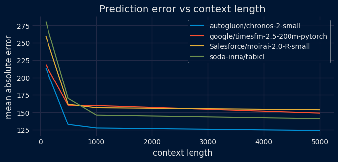
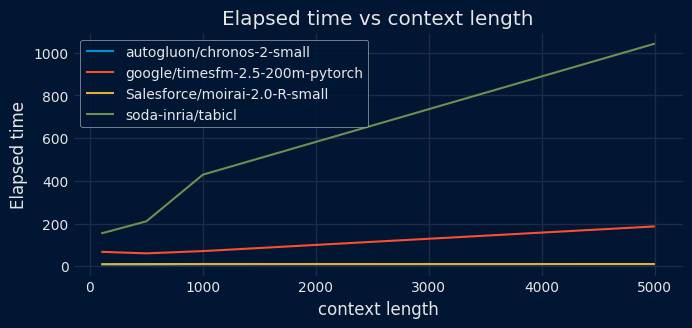
Selection of context length
As described in the Impact of the context length section, the context length has a direct effect on both the model's predictive accuracy and the computation time required to generate forecasts. Furthermore, because the context must be sent to the model every time a prediction is made, it also increases the amount of data transferred when the model is deployed in production. It is therefore important to identify the optimal context length that strikes a good balance between predictive accuracy and inference time.
The following code shows how to evaluate the impact of the context length on the predictive accuracy and inference time of a foundation model. The example uses the Amazon Chronos-2-small model, but the same approach can be applied to any other foundation model supported by skforecast.
# Influence of the context length in the forecasting accuracy and speed
# ==============================================================================
model_id = 'autogluon/chronos-2-small'
context_lengths = [100, 500, 1000, 5000]

model_ids_allow_exog = {
    'autogluon/chronos-2-small', 'soda-inria/tabicl', 'priorlabs/tabpfn-ts', 'theforecastingcompany/t0-alpha'
}
if model_id in model_ids_allow_exog:
    exog = data[["Temperature", "Holiday"]]
else:
    exog = None

cv = TimeSeriesFold(
         steps              = 24,
         initial_train_size = len(data.loc[:end_train]),
         refit              = False
     )

results_metrics = []
results_elapsed_time = []
for context_length in context_lengths:

    estimator = FoundationModel(model_id=model_id, context_length=context_length)
    forecaster = ForecasterFoundation(estimator=estimator)

    start = time.perf_counter()
    metrics, backtest_predictions = backtesting_foundation(
        forecaster        = forecaster,
        series            = data['Demand'],
        exog              = exog,
        cv                = cv,
        metric            = 'mean_absolute_error',
        suppress_warnings = True,
        show_progress     = False
    )
    elapsed_time = time.perf_counter() - start

    results_metrics.append(metrics.at[0, 'mean_absolute_error'])
    results_elapsed_time.append(elapsed_time)

results = pd.DataFrame(
    {
        'metric': results_metrics,
        'elapsed_time': results_elapsed_time
    },
    index=context_lengths
)
results
Loading weights: 0%| | 0/92 [00:00<?, ?it/s]
Loading weights: 0%| | 0/92 [00:00<?, ?it/s]
Loading weights: 0%| | 0/92 [00:00<?, ?it/s]
Loading weights: 0%| | 0/92 [00:00<?, ?it/s]
| metric | elapsed_time | |
|---|---|---|
| 100 | 214.318950 | 2.500289 |
| 500 | 171.266983 | 2.885307 |
| 1000 | 155.492158 | 3.365345 |
| 5000 | 158.398215 | 7.331956 |
# Plot results
# ==============================================================================
fig, ax = plt.subplots(figsize=(7, 3))
results['metric'].plot(ax = ax)
ax.set_title("Prediction error vs context length")
ax.set_xlabel("context length")
ax.set_ylabel("mean absolute error")

fig, ax = plt.subplots(figsize=(7, 3))
results['elapsed_time'].plot(ax = ax)
ax.set_title("Elapsed time vs context length")
ax.set_xlabel("context length")
ax.set_ylabel("Elapsed time");

