Direct multi-step forecaster¶

This strategy, commonly known as direct multistep forecasting, is computationally more expensive than the recursive since it requires training several models. However, in some scenarios, it achieves better results. This type of model can be obtained with the ForecasterAutoregDirect class and can also include one or multiple exogenous variables.

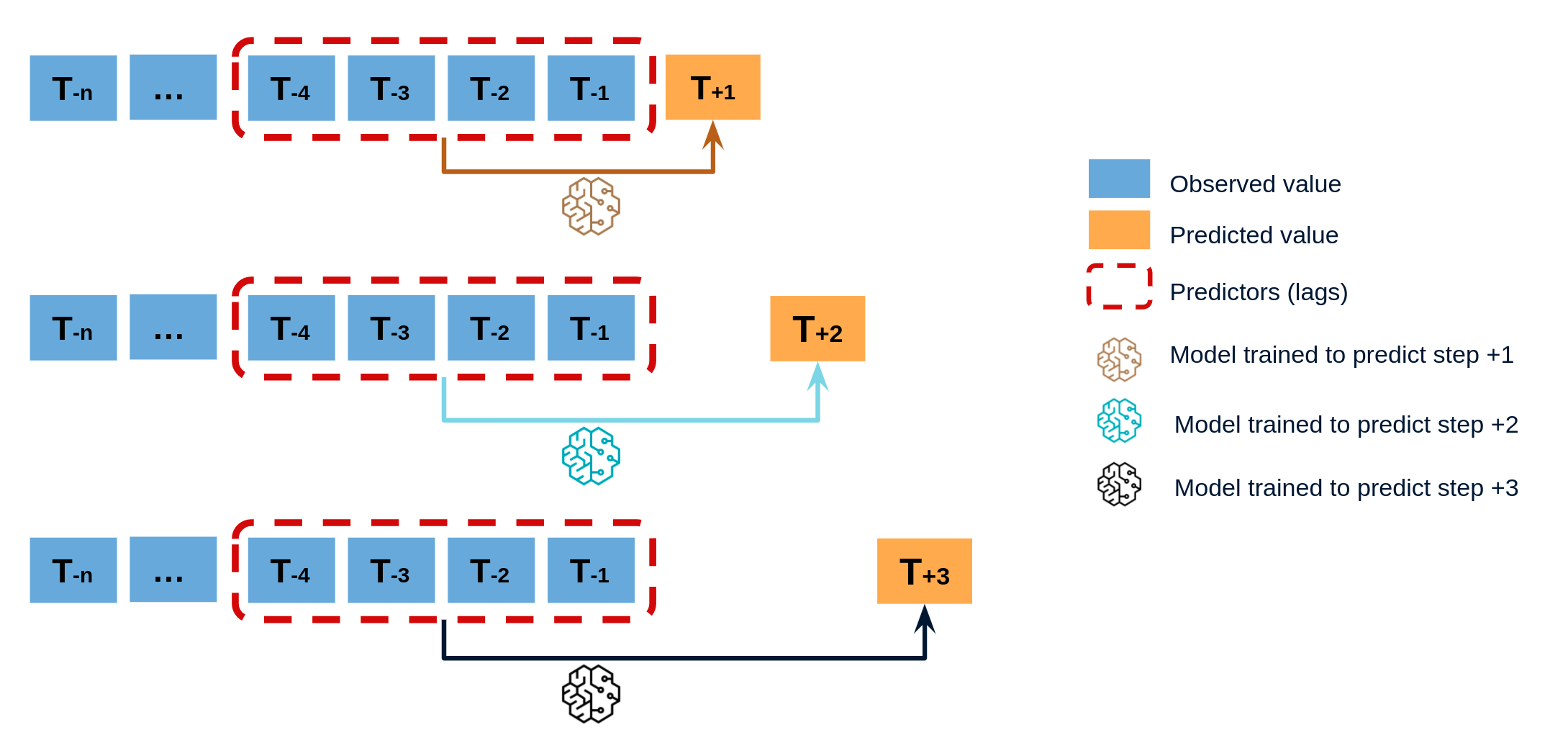
Direct multi-step forecasting is a time series forecasting strategy in which a separate model is trained to predict each step in the forecast horizon. This is in contrast to recursive multi-step forecasting, where a single model is used to make predictions for all future time steps by recursively using its own output as input.

Direct multi-step forecasting can be more computationally expensive than recursive forecasting since it requires training multiple models. However, it can often achieve better accuracy in certain scenarios, particularly when there are complex patterns and dependencies in the data that are difficult to capture with a single model.

Direct multi-step forecasting can be performed using the ForecasterAutoregDirect class, which can also incorporate one or multiple exogenous variables to improve the accuracy of the forecasts.

Diagram of direct multi-step forecasting.

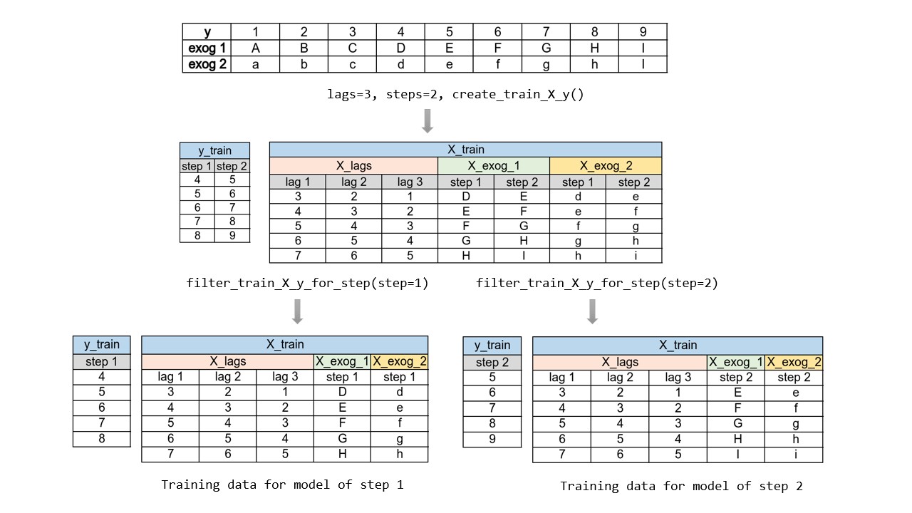
To train a ForecasterAutoregDirect a different training matrix is created for each model.

Transformation of a time series into matrices to train a direct multi-step forecasting model.

  Note

Starting from version skforecast 0.9.0, the ForecasterAutoregDirect now includes the n_jobs parameter, allowing multi-process parallelization. This allows to train regressors for all steps simultaneously.

The benefits of parallelization depend on several factors, including the regressor used, the number of fits to be performed, and the volume of data involved. When the n_jobs parameter is set to 'auto', the level of parallelization is automatically selected based on heuristic rules that aim to choose the best option for each scenario.

Libraries¶

In [1]:

# Libraries
# ==============================================================================
import numpy as np
import pandas as pd
import matplotlib.pyplot as plt
from skforecast.ForecasterAutoregDirect import ForecasterAutoregDirect
from sklearn.linear_model import Ridge
from sklearn.metrics import mean_squared_error

# Libraries # ============================================================================== import numpy as np import pandas as pd import matplotlib.pyplot as plt from skforecast.ForecasterAutoregDirect import ForecasterAutoregDirect from sklearn.linear_model import Ridge from sklearn.metrics import mean_squared_error

Data¶

In [2]:

# Download data
# ==============================================================================
url = (
    'https://raw.githubusercontent.com/JoaquinAmatRodrigo/skforecast/master/'
    'data/h2o.csv'
)
data = pd.read_csv(url, sep=',', header=0, names=['y', 'datetime'])

# Data preprocessing
# ==============================================================================
data['datetime'] = pd.to_datetime(data['datetime'], format='%Y-%m-%d')
data = data.set_index('datetime')
data = data.asfreq('MS')
data = data['y']
data = data.sort_index()

# Split train-test
# ==============================================================================
steps = 36
data_train = data[:-steps]
data_test  = data[-steps:]

# Plot
# ==============================================================================
fig, ax = plt.subplots(figsize=(6, 3))
data_train.plot(ax=ax, label='train')
data_test.plot(ax=ax, label='test')
ax.legend();

# Download data # ============================================================================== url = ( 'https://raw.githubusercontent.com/JoaquinAmatRodrigo/skforecast/master/' 'data/h2o.csv' ) data = pd.read_csv(url, sep=',', header=0, names=['y', 'datetime']) # Data preprocessing # ============================================================================== data['datetime'] = pd.to_datetime(data['datetime'], format='%Y-%m-%d') data = data.set_index('datetime') data = data.asfreq('MS') data = data['y'] data = data.sort_index() # Split train-test # ============================================================================== steps = 36 data_train = data[:-steps] data_test = data[-steps:] # Plot # ============================================================================== fig, ax = plt.subplots(figsize=(6, 3)) data_train.plot(ax=ax, label='train') data_test.plot(ax=ax, label='test') ax.legend();

Create and train forecaster¶

In [3]:

# Create and fit forecaster
# ==============================================================================
forecaster = ForecasterAutoregDirect(
                 regressor     = Ridge(),
                 steps         = 36,
                 lags          = 15,
                 transformer_y = None,
                 n_jobs        = 'auto'
             )

forecaster.fit(y=data_train)
forecaster

# Create and fit forecaster # ============================================================================== forecaster = ForecasterAutoregDirect( regressor = Ridge(), steps = 36, lags = 15, transformer_y = None, n_jobs = 'auto' ) forecaster.fit(y=data_train) forecaster

Out[3]:

======================= 
ForecasterAutoregDirect 
======================= 
Regressor: Ridge() 
Lags: [ 1  2  3  4  5  6  7  8  9 10 11 12 13 14 15] 
Transformer for y: None 
Transformer for exog: None 
Weight function included: False 
Window size: 15 
Maximum steps predicted: 36 
Exogenous included: False 
Type of exogenous variable: None 
Exogenous variables names: None 
Training range: [Timestamp('1991-07-01 00:00:00'), Timestamp('2005-06-01 00:00:00')] 
Training index type: DatetimeIndex 
Training index frequency: MS 
Regressor parameters: {'alpha': 1.0, 'copy_X': True, 'fit_intercept': True, 'max_iter': None, 'positive': False, 'random_state': None, 'solver': 'auto', 'tol': 0.0001} 
fit_kwargs: {} 
Creation date: 2023-07-08 13:51:10 
Last fit date: 2023-07-08 13:51:10 
Skforecast version: 0.9.0 
Python version: 3.11.4 
Forecaster id: None 

Prediction¶

When predicting, the value of steps must be less than or equal to the value of steps defined when initializing the forecaster. Starts at 1.

• If int only steps within the range of 1 to int are predicted.

• If list of int. Only the steps contained in the list are predicted.

• If None as many steps are predicted as were defined at initialization.

In [4]:

# Predict
# ==============================================================================
# Predict only a subset of steps
predictions = forecaster.predict(steps=[1, 5])
display(predictions)

# Predict # ============================================================================== # Predict only a subset of steps predictions = forecaster.predict(steps=[1, 5]) display(predictions)

2005-07-01    0.952051
2005-11-01    1.179922
Name: pred, dtype: float64

In [5]:

# Predict all steps defined in the initialization.
predictions = forecaster.predict()
display(predictions.head(3))

# Predict all steps defined in the initialization. predictions = forecaster.predict() display(predictions.head(3))

2005-07-01    0.952051
2005-08-01    1.004145
2005-09-01    1.114590
Name: pred, dtype: float64

In [6]:

# Plot predictions
# ==============================================================================
fig, ax = plt.subplots(figsize=(6, 3))
data_train.plot(ax=ax, label='train')
data_test.plot(ax=ax, label='test')
predictions.plot(ax=ax, label='predictions')
ax.legend();

# Plot predictions # ============================================================================== fig, ax = plt.subplots(figsize=(6, 3)) data_train.plot(ax=ax, label='train') data_test.plot(ax=ax, label='test') predictions.plot(ax=ax, label='predictions') ax.legend();

In [7]:

# Prediction error
# ==============================================================================
predictions = forecaster.predict(steps=36)

error_mse = mean_squared_error(
                y_true = data_test,
                y_pred = predictions
            )
            
print(f"Test error (mse): {error_mse}")

# Prediction error # ============================================================================== predictions = forecaster.predict(steps=36) error_mse = mean_squared_error( y_true = data_test, y_pred = predictions ) print(f"Test error (mse): {error_mse}")

Test error (mse): 0.008419597278831965

Feature importances¶

Since ForecasterAutoregDirect fits one model per step, it is necessary to specify from which model retrieves its feature importances.

In [8]:

forecaster.get_feature_importances(step=1)

forecaster.get_feature_importances(step=1)

Out[8]:

	feature	importance
0	lag_1	0.139299
1	lag_2	0.051089
2	lag_3	0.044192
3	lag_4	-0.019868
4	lag_5	-0.017935
5	lag_6	-0.013233
6	lag_7	-0.021063
7	lag_8	-0.012591
8	lag_9	0.011918
9	lag_10	0.020511
10	lag_11	0.154030
11	lag_12	0.551652
12	lag_13	0.057513
13	lag_14	-0.071071
14	lag_15	-0.035237

Extract training matrices¶

Two steps are needed to extract the training matrices. One to create the whole training matrix and a second one to subset the data needed for each model (step).

In [9]:

# Create the whole train matrix
X, y = forecaster.create_train_X_y(data_train)

# Extract X and y to train the model for step 1
X_1, y_1 = forecaster.filter_train_X_y_for_step(
               step          = 1,
               X_train       = X,
               y_train       = y,
               remove_suffix = False
           )

X_1.head(4)

# Create the whole train matrix X, y = forecaster.create_train_X_y(data_train) # Extract X and y to train the model for step 1 X_1, y_1 = forecaster.filter_train_X_y_for_step( step = 1, X_train = X, y_train = y, remove_suffix = False ) X_1.head(4)

Out[9]:

	lag_1	lag_2	lag_3	lag_4	lag_5	lag_6	lag_7	lag_8	lag_9	lag_10	lag_11	lag_12	lag_13	lag_14	lag_15
datetime
1992-10-01	0.534761	0.475463	0.483389	0.410534	0.361801	0.379808	0.351348	0.336220	0.660119	0.602652	0.502369	0.492543	0.432159	0.400906	0.429795
1992-11-01	0.568606	0.534761	0.475463	0.483389	0.410534	0.361801	0.379808	0.351348	0.336220	0.660119	0.602652	0.502369	0.492543	0.432159	0.400906
1992-12-01	0.595223	0.568606	0.534761	0.475463	0.483389	0.410534	0.361801	0.379808	0.351348	0.336220	0.660119	0.602652	0.502369	0.492543	0.432159
1993-01-01	0.771258	0.595223	0.568606	0.534761	0.475463	0.483389	0.410534	0.361801	0.379808	0.351348	0.336220	0.660119	0.602652	0.502369	0.492543

In [10]:

y_1.head(4)

y_1.head(4)

Out[10]:

datetime
1992-10-01    0.568606
1992-11-01    0.595223
1992-12-01    0.771258
1993-01-01    0.751503
Freq: MS, Name: y_step_1, dtype: float64

In [11]:

%%html
<style>
.jupyter-wrapper .jp-CodeCell .jp-Cell-inputWrapper .jp-InputPrompt {display: none;}
</style>

%%html