Independent multi-series forecasting¶

In univariate time series forecasting, a single time series is modeled as a linear or nonlinear combination of its lags, where past values of the series are used to forecast its future. In multi-series forecasting, two or more time series are modeled together using a single model.

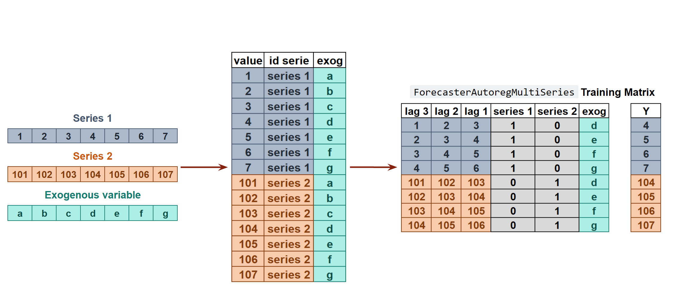
In independent multi-series forecasting a single model is trained for all time series, but each time series remains independent of the others, meaning that past values of one series are not used as predictors of other series. However, modeling them together is useful because the series may follow the same intrinsic pattern regarding their past and future values. For instance, the sales of products A and B in the same store may not be related, but they follow the same dynamics, that of the store.

Transformation of two time series and an exogenous variable into the matrices needed to train a machine learning model in a multi-series context.

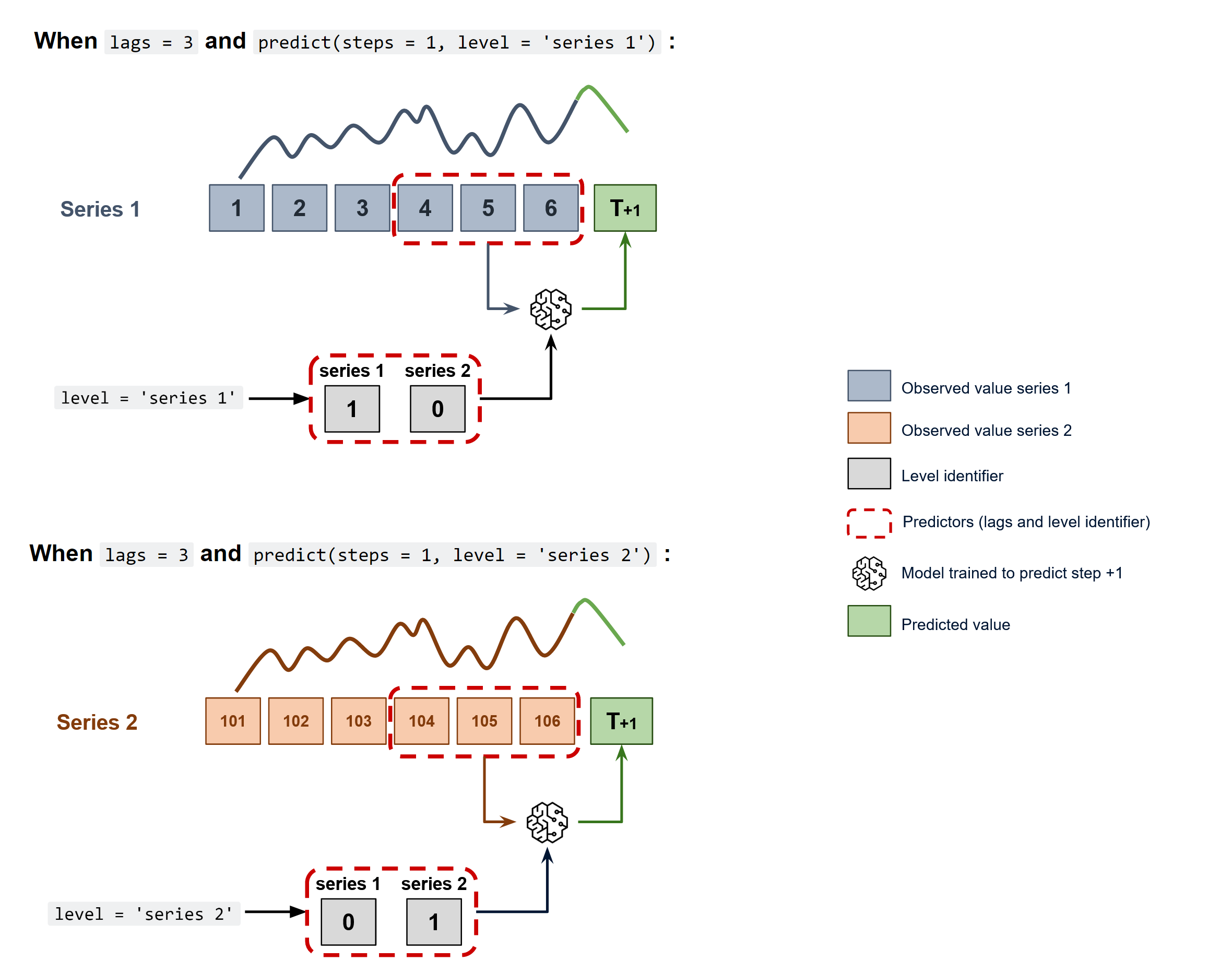
To predict the next n steps, the strategy of recursive multi-step forecasting is applied, with the only difference being that the series name for which to estimate the predictions needs to be indicated.

Diagram of recursive forecasting with multiple independent time series.

Using the ForecasterAutoregMultiSeries and ForecasterAutoregMultiSeriesCustom classes, it is possible to easily build machine learning models for independent multi-series forecasting.

  Note

See ForecasterAutoregMultiVariate for dependent multi-series forecasting (multivariate time series).

Libraries¶

In [1]:

# Libraries
# ==============================================================================
import numpy as np
import pandas as pd
import matplotlib.pyplot as plt
from sklearn.preprocessing import StandardScaler
from sklearn.linear_model import Ridge
from sklearn.metrics import mean_absolute_error

from skforecast.ForecasterAutoregMultiSeries import ForecasterAutoregMultiSeries
from skforecast.model_selection_multiseries import backtesting_forecaster_multiseries
from skforecast.model_selection_multiseries import grid_search_forecaster_multiseries

# Libraries # ============================================================================== import numpy as np import pandas as pd import matplotlib.pyplot as plt from sklearn.preprocessing import StandardScaler from sklearn.linear_model import Ridge from sklearn.metrics import mean_absolute_error from skforecast.ForecasterAutoregMultiSeries import ForecasterAutoregMultiSeries from skforecast.model_selection_multiseries import backtesting_forecaster_multiseries from skforecast.model_selection_multiseries import grid_search_forecaster_multiseries

Data¶

In [2]:

# Data download
# ==============================================================================
url = (
       'https://raw.githubusercontent.com/JoaquinAmatRodrigo/skforecast/master/'
       'data/simulated_items_sales.csv'
)
data = pd.read_csv(url, sep=',')

# Data preparation
# ==============================================================================
data['date'] = pd.to_datetime(data['date'], format='%Y-%m-%d')
data = data.set_index('date')
data = data.asfreq('D')
data = data.sort_index()
data.head()

# Data download # ============================================================================== url = ( 'https://raw.githubusercontent.com/JoaquinAmatRodrigo/skforecast/master/' 'data/simulated_items_sales.csv' ) data = pd.read_csv(url, sep=',') # Data preparation # ============================================================================== data['date'] = pd.to_datetime(data['date'], format='%Y-%m-%d') data = data.set_index('date') data = data.asfreq('D') data = data.sort_index() data.head()

Out[2]:

	item_1	item_2	item_3
date
2012-01-01	8.253175	21.047727	19.429739
2012-01-02	22.777826	26.578125	28.009863
2012-01-03	27.549099	31.751042	32.078922
2012-01-04	25.895533	24.567708	27.252276
2012-01-05	21.379238	18.191667	20.357737

In [3]:

# Split data into train-val-test
# ==============================================================================
end_train = '2014-07-15 23:59:00'
data_train = data.loc[:end_train, :].copy()
data_test  = data.loc[end_train:, :].copy()

print(
    f"Train dates : {data_train.index.min()} --- {data_train.index.max()}   "
    f"(n={len(data_train)})"
)
print(
    f"Test dates  : {data_test.index.min()} --- {data_test.index.max()}   "
    f"(n={len(data_test)})"
)

# Split data into train-val-test # ============================================================================== end_train = '2014-07-15 23:59:00' data_train = data.loc[:end_train, :].copy() data_test = data.loc[end_train:, :].copy() print( f"Train dates : {data_train.index.min()} --- {data_train.index.max()} " f"(n={len(data_train)})" ) print( f"Test dates : {data_test.index.min()} --- {data_test.index.max()} " f"(n={len(data_test)})" )

Train dates : 2012-01-01 00:00:00 --- 2014-07-15 00:00:00   (n=927)
Test dates  : 2014-07-16 00:00:00 --- 2015-01-01 00:00:00   (n=170)

In [4]:

# Plot time series
# ==============================================================================
fig, axes = plt.subplots(nrows=3, ncols=1, figsize=(9, 5), sharex=True)

data_train['item_1'].plot(label='train', ax=axes[0])
data_test['item_1'].plot(label='test', ax=axes[0])
axes[0].set_xlabel('')
axes[0].set_ylabel('sales')
axes[0].set_title('Item 1')
axes[0].legend()

data_train['item_2'].plot(label='train', ax=axes[1])
data_test['item_2'].plot(label='test', ax=axes[1])
axes[1].set_xlabel('')
axes[1].set_ylabel('sales')
axes[1].set_title('Item 2')

data_train['item_3'].plot(label='train', ax=axes[2])
data_test['item_3'].plot(label='test', ax=axes[2])
axes[2].set_xlabel('')
axes[2].set_ylabel('sales')
axes[2].set_title('Item 3')

fig.tight_layout()
plt.show();

# Plot time series # ============================================================================== fig, axes = plt.subplots(nrows=3, ncols=1, figsize=(9, 5), sharex=True) data_train['item_1'].plot(label='train', ax=axes[0]) data_test['item_1'].plot(label='test', ax=axes[0]) axes[0].set_xlabel('') axes[0].set_ylabel('sales') axes[0].set_title('Item 1') axes[0].legend() data_train['item_2'].plot(label='train', ax=axes[1]) data_test['item_2'].plot(label='test', ax=axes[1]) axes[1].set_xlabel('') axes[1].set_ylabel('sales') axes[1].set_title('Item 2') data_train['item_3'].plot(label='train', ax=axes[2]) data_test['item_3'].plot(label='test', ax=axes[2]) axes[2].set_xlabel('') axes[2].set_ylabel('sales') axes[2].set_title('Item 3') fig.tight_layout() plt.show();

Train and predict ForecasterAutoregMultiSeries¶

In [5]:

# Create and fit forecaster multi series
# ==============================================================================
forecaster = ForecasterAutoregMultiSeries(
                 regressor          = Ridge(random_state=123),
                 lags               = 24,
                 transformer_series = None,
                 transformer_exog   = None,
                 weight_func        = None,
                 series_weights     = None
             )

forecaster.fit(series=data_train)
forecaster

# Create and fit forecaster multi series # ============================================================================== forecaster = ForecasterAutoregMultiSeries( regressor = Ridge(random_state=123), lags = 24, transformer_series = None, transformer_exog = None, weight_func = None, series_weights = None ) forecaster.fit(series=data_train) forecaster

Out[5]:

============================ 
ForecasterAutoregMultiSeries 
============================ 
Regressor: Ridge(random_state=123) 
Lags: [ 1  2  3  4  5  6  7  8  9 10 11 12 13 14 15 16 17 18 19 20 21 22 23 24] 
Transformer for series: None 
Transformer for exog: None 
Window size: 24 
Series levels (names): ['item_1', 'item_2', 'item_3'] 
Series weights: None 
Weight function included: False 
Exogenous included: False 
Type of exogenous variable: None 
Exogenous variables names: None 
Training range: [Timestamp('2012-01-01 00:00:00'), Timestamp('2014-07-15 00:00:00')] 
Training index type: DatetimeIndex 
Training index frequency: D 
Regressor parameters: {'alpha': 1.0, 'copy_X': True, 'fit_intercept': True, 'max_iter': None, 'positive': False, 'random_state': 123, 'solver': 'auto', 'tol': 0.0001} 
fit_kwargs: {} 
Creation date: 2023-05-19 21:11:58 
Last fit date: 2023-05-19 21:11:58 
Skforecast version: 0.8.0 
Python version: 3.9.13 
Forecaster id: None 

Two methods can be use to predict the next n steps: predict() or predict_interval(). The argument levels is used to indicate for which series estimate predictions. If None all series will be predicted.

In [6]:

# Predict and predict_interval
# ==============================================================================
steps = 24

# Predictions for item_1
predictions_item_1 = forecaster.predict(steps=steps, levels='item_1')
display(predictions_item_1.head(3))

# Interval predictions for item_1 and item_2
predictions_intervals = forecaster.predict_interval(steps=steps, levels=['item_1', 'item_2'])
display(predictions_intervals.head(3))

# Predict and predict_interval # ============================================================================== steps = 24 # Predictions for item_1 predictions_item_1 = forecaster.predict(steps=steps, levels='item_1') display(predictions_item_1.head(3)) # Interval predictions for item_1 and item_2 predictions_intervals = forecaster.predict_interval(steps=steps, levels=['item_1', 'item_2']) display(predictions_intervals.head(3))

	item_1
2014-07-16	25.497376
2014-07-17	24.866972
2014-07-18	24.281173

	item_1	item_1_lower_bound	item_1_upper_bound	item_2	item_2_lower_bound	item_2_upper_bound
2014-07-16	25.497376	23.220087	28.226068	10.694506	7.093046	15.518896
2014-07-17	24.866972	22.141168	27.389805	11.080091	6.467676	16.534679
2014-07-18	24.281173	21.688393	26.981395	11.490882	7.077863	16.762530

Backtesting Multi Series¶

As in the predict method, the levels at which backtesting is performed must be indicated. The argument can also be set to None to perform backtesting at all levels.

In [7]:

# Backtesting Multi Series
# ==============================================================================
metrics_levels, backtest_predictions = backtesting_forecaster_multiseries(
                                           forecaster            = forecaster,
                                           series                = data,
                                           levels                = None,
                                           steps                 = 24,
                                           metric                = 'mean_absolute_error',
                                           initial_train_size    = len(data_train),
                                           fixed_train_size      = True,
                                           gap                   = 0,
                                           allow_incomplete_fold = True,
                                           refit                 = True,
                                           verbose               = False,
                                           show_progress         = True
                                       )

print("Backtest metrics")
display(metrics_levels)
print("")
print("Backtest predictions")
backtest_predictions.head(4)

# Backtesting Multi Series # ============================================================================== metrics_levels, backtest_predictions = backtesting_forecaster_multiseries( forecaster = forecaster, series = data, levels = None, steps = 24, metric = 'mean_absolute_error', initial_train_size = len(data_train), fixed_train_size = True, gap = 0, allow_incomplete_fold = True, refit = True, verbose = False, show_progress = True ) print("Backtest metrics") display(metrics_levels) print("") print("Backtest predictions") backtest_predictions.head(4)

100%|██████████| 8/8 [00:00<00:00, 101.26it/s]

Backtest metrics

	levels	mean_absolute_error
0	item_1	1.360675
1	item_2	2.332392
2	item_3	3.155592

Backtest predictions

Out[7]:

	item_1	item_2	item_3
2014-07-16	25.497376	10.694506	11.275026
2014-07-17	24.866972	11.080091	11.313510
2014-07-18	24.281173	11.490882	13.030112
2014-07-19	23.515499	11.548922	13.378282

Hyperparameter tuning and lags selection Multi Series¶

Functions grid_search_forecaster_multiseries and random_search_forecaster_multiseries in the module model_selection_multiseries allow for lag and hyperparameter optimization. The optimization is performed in the same way as in the other forecasters, see the user guide here, except for the levels argument:

• levels: level(s) at which the forecaster is optimized, for example:

  • If levels = ['item_1', 'item_2', 'item_3'] (Same as levels = None), the function will search for the lags and hyperparameters that minimize the average error of the predictions of all the time series. The resulting metric will be the average of all levels.

  • If levels = 'item_1' (Same as levels = ['item_1']), the function will search for the lags and hyperparameters that minimize the error of the item_1 predictions. The resulting metric will be the one calculated for item_1.

The following example shows how to use grid_search_forecaster_multiseries to find the best lags and model hyperparameters for all time series:

In [8]:

# Create Forecaster multi series
# ==============================================================================
forecaster = ForecasterAutoregMultiSeries(
                 regressor          = Ridge(random_state=123),
                 lags               = 24,
                 transformer_series = StandardScaler(),
                 transformer_exog   = None,
                 weight_func        = None,
                 series_weights     = None
             )

# Create Forecaster multi series # ============================================================================== forecaster = ForecasterAutoregMultiSeries( regressor = Ridge(random_state=123), lags = 24, transformer_series = StandardScaler(), transformer_exog = None, weight_func = None, series_weights = None )

In [9]:

# Grid search Multi Series
# ==============================================================================
lags_grid = [24, 48]
param_grid = {'alpha': [0.01, 0.1, 1]}

levels = ['item_1', 'item_2', 'item_3']

results = grid_search_forecaster_multiseries(
              forecaster          = forecaster,
              series              = data,
              exog                = None,
              levels              = levels,
              lags_grid           = lags_grid,
              param_grid          = param_grid,
              steps               = 24,
              metric              = 'mean_absolute_error',
              initial_train_size  = len(data_train),
              refit               = True,
              fixed_train_size    = True,
              return_best         = False,
              verbose             = False
          )

results

# Grid search Multi Series # ============================================================================== lags_grid = [24, 48] param_grid = {'alpha': [0.01, 0.1, 1]} levels = ['item_1', 'item_2', 'item_3'] results = grid_search_forecaster_multiseries( forecaster = forecaster, series = data, exog = None, levels = levels, lags_grid = lags_grid, param_grid = param_grid, steps = 24, metric = 'mean_absolute_error', initial_train_size = len(data_train), refit = True, fixed_train_size = True, return_best = False, verbose = False ) results

6 models compared for 3 level(s). Number of iterations: 6.

lags grid: 100%|██████████| 2/2 [00:00<00:00,  2.34it/s]

Out[9]:

	levels	lags	params	mean_absolute_error	alpha
5	[item_1, item_2, item_3]	[1, 2, 3, 4, 5, 6, 7, 8, 9, 10, 11, 12, 13, 14...	{'alpha': 1}	2.207648	1.00
4	[item_1, item_2, item_3]	[1, 2, 3, 4, 5, 6, 7, 8, 9, 10, 11, 12, 13, 14...	{'alpha': 0.1}	2.207700	0.10
3	[item_1, item_2, item_3]	[1, 2, 3, 4, 5, 6, 7, 8, 9, 10, 11, 12, 13, 14...	{'alpha': 0.01}	2.207706	0.01
2	[item_1, item_2, item_3]	[1, 2, 3, 4, 5, 6, 7, 8, 9, 10, 11, 12, 13, 14...	{'alpha': 1}	2.335039	1.00
1	[item_1, item_2, item_3]	[1, 2, 3, 4, 5, 6, 7, 8, 9, 10, 11, 12, 13, 14...	{'alpha': 0.1}	2.335149	0.10
0	[item_1, item_2, item_3]	[1, 2, 3, 4, 5, 6, 7, 8, 9, 10, 11, 12, 13, 14...	{'alpha': 0.01}	2.335161	0.01

Weights in multi-series¶

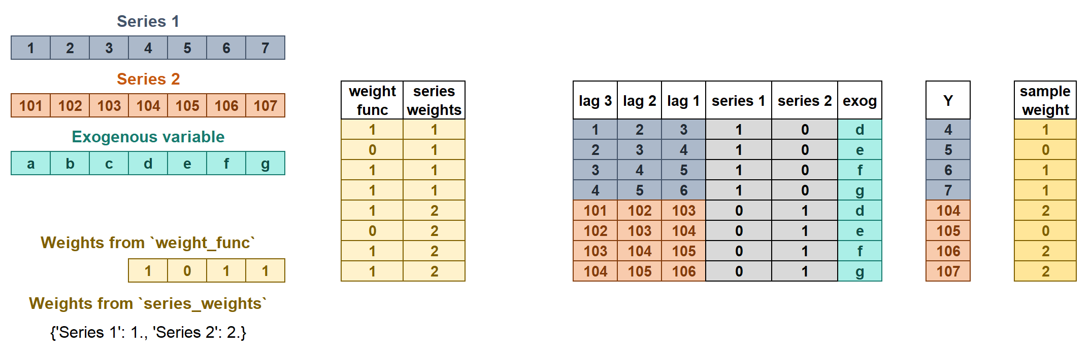
The weights are used to control the influence that each observation has on the training of the model. ForecasterAutoregMultiseries accepts two types of weights:

• series_weights controls the relative importance of each series. If a series has twice as much weight as the others, the observations of that series influence the training twice as much. The higher the weight of a series relative to the others, the more the model will focus on trying to learn that series.

• weight_func controls the relative importance of each observation according to its index value. For example, a function that assigns a lower weight to certain dates.

If the two types of weights are indicated, they are multiplied to create the final weights. The resulting sample_weight cannot have negative values.

• series_weights is a dict of the form {'series_column_name': float}. If a series is used during fit and is not present in series_weights, it will have a weight of 1.

• weight_func is a function that defines the individual weights of each sample based on the index.

  • If it is a callable, the same function will apply to all series.

  • If it is a dict of the form {'series_column_name': callable}, a different function can be used for each series. A weight of 1 is given to all series not present in weight_func.

In [10]:

# Weights in Multi-Series
# ==============================================================================
def custom_weights(index):
    """
    Return 0 if index is between '2013-01-01' and '2013-01-31', 1 otherwise.
    """
    weights = np.where(
                  (index >= '2013-01-01') & (index <= '2013-01-31'),
                   0,
                   1
              )
    
    return weights

forecaster = ForecasterAutoregMultiSeries(
                 regressor          = Ridge(random_state=123),
                 lags               = 24,
                 transformer_series = None,
                 transformer_exog   = None,
                 weight_func        = custom_weights,
                 series_weights     = {'item_1': 1., 'item_2': 2., 'item_3': 1.} # Same as {'item_2': 2.}
             )

forecaster.fit(series=data_train)
forecaster.predict(steps=24).head(3)

# Weights in Multi-Series # ============================================================================== def custom_weights(index): """ Return 0 if index is between '2013-01-01' and '2013-01-31', 1 otherwise. """ weights = np.where( (index >= '2013-01-01') & (index <= '2013-01-31'), 0, 1 ) return weights forecaster = ForecasterAutoregMultiSeries( regressor = Ridge(random_state=123), lags = 24, transformer_series = None, transformer_exog = None, weight_func = custom_weights, series_weights = {'item_1': 1., 'item_2': 2., 'item_3': 1.} # Same as {'item_2': 2.} ) forecaster.fit(series=data_train) forecaster.predict(steps=24).head(3)

Out[10]:

	item_1	item_2	item_3
2014-07-16	25.547560	10.527454	11.195018
2014-07-17	24.779779	10.987891	11.424717
2014-07-18	24.182702	11.375158	13.090853

  Warning

The weight_func and series_weights arguments will be ignored if the regressor does not accept sample_weight in its fit method.

The source code of the weight_func added to the forecaster is stored in the argument source_code_weight_func. If weight_func is a dict, it will be a dict of the form {'series_column_name': source_code_weight_func} .

In [11]:

print(forecaster.source_code_weight_func)

print(forecaster.source_code_weight_func)

def custom_weights(index):
    """
    Return 0 if index is between '2013-01-01' and '2013-01-31', 1 otherwise.
    """
    weights = np.where(
                  (index >= '2013-01-01') & (index <= '2013-01-31'),
                   0,
                   1
              )
    
    return weights

Scikit-learn transformers in multi-series¶

Learn more about using scikit-learn transformers with skforecast.

• If transformer_series is a transformer the same transformation will be applied to all series.
• If transformer_series is a dict a different transformation can be set for each series. Series not present in the dict will not have any transformation applied to them.

In [12]:

forecaster = ForecasterAutoregMultiSeries(
                 regressor          = Ridge(random_state=123),
                 lags               = 24,
                 transformer_series = {'item_1': StandardScaler(), 'item_2': StandardScaler()},
                 transformer_exog   = None,
                 weight_func        = None,
                 series_weights     = None
             )

forecaster.fit(series=data_train)
forecaster

forecaster = ForecasterAutoregMultiSeries( regressor = Ridge(random_state=123), lags = 24, transformer_series = {'item_1': StandardScaler(), 'item_2': StandardScaler()}, transformer_exog = None, weight_func = None, series_weights = None ) forecaster.fit(series=data_train) forecaster

c:\Users\jaesc2\Miniconda3\envs\skforecast\lib\site-packages\skforecast\ForecasterAutoregMultiSeries\ForecasterAutoregMultiSeries.py:453: IgnoredArgumentWarning: {'item_3'} not present in `transformer_series`. No transformation is applied to these series. 
 You can suppress this warning using: warnings.simplefilter('ignore', category=IgnoredArgumentWarning)
  warnings.warn(

Out[12]:

============================ 
ForecasterAutoregMultiSeries 
============================ 
Regressor: Ridge(random_state=123) 
Lags: [ 1  2  3  4  5  6  7  8  9 10 11 12 13 14 15 16 17 18 19 20 21 22 23 24] 
Transformer for series: {'item_1': StandardScaler(), 'item_2': StandardScaler()} 
Transformer for exog: None 
Window size: 24 
Series levels (names): ['item_1', 'item_2', 'item_3'] 
Series weights: None 
Weight function included: False 
Exogenous included: False 
Type of exogenous variable: None 
Exogenous variables names: None 
Training range: [Timestamp('2012-01-01 00:00:00'), Timestamp('2014-07-15 00:00:00')] 
Training index type: DatetimeIndex 
Training index frequency: D 
Regressor parameters: {'alpha': 1.0, 'copy_X': True, 'fit_intercept': True, 'max_iter': None, 'positive': False, 'random_state': 123, 'solver': 'auto', 'tol': 0.0001} 
fit_kwargs: {} 
Creation date: 2023-05-19 21:12:01 
Last fit date: 2023-05-19 21:12:01 
Skforecast version: 0.8.0 
Python version: 3.9.13 
Forecaster id: None 

Compare multiple metrics¶

All three functions (backtesting_forecaster_multiseries, grid_search_forecaster_multiseries, and random_search_forecaster_multiseries) allow the calculation of multiple metrics for each forecaster configuration if a list is provided. This list may include custom metrics and the best model selection is done based on the first metric of the list.

In [13]:

# Grid search Multi-Series with multiple metrics
# ==============================================================================
forecaster = ForecasterAutoregMultiSeries(
                 regressor          = Ridge(random_state=123),
                 lags               = 24
             )

def custom_metric(y_true, y_pred):
    """
    Calculate the mean absolute error using only the predicted values of the last
    3 months of the year.
    """
    mask = y_true.index.month.isin([10, 11, 12])
    metric = mean_absolute_error(y_true[mask], y_pred[mask])
    
    return metric

lags_grid = [24, 48]
param_grid = {'alpha': [0.01, 0.1, 1]}

results = grid_search_forecaster_multiseries(
              forecaster          = forecaster,
              series              = data,
              lags_grid           = lags_grid,
              param_grid          = param_grid,
              steps               = 24,
              metric              = [mean_absolute_error, custom_metric, 'mean_squared_error'],
              initial_train_size  = len(data_train),
              fixed_train_size    = True,
              levels              = None,
              exog                = None,
              refit               = True,
              return_best         = False,
              verbose             = False
          )

results

# Grid search Multi-Series with multiple metrics # ============================================================================== forecaster = ForecasterAutoregMultiSeries( regressor = Ridge(random_state=123), lags = 24 ) def custom_metric(y_true, y_pred): """ Calculate the mean absolute error using only the predicted values of the last 3 months of the year. """ mask = y_true.index.month.isin([10, 11, 12]) metric = mean_absolute_error(y_true[mask], y_pred[mask]) return metric lags_grid = [24, 48] param_grid = {'alpha': [0.01, 0.1, 1]} results = grid_search_forecaster_multiseries( forecaster = forecaster, series = data, lags_grid = lags_grid, param_grid = param_grid, steps = 24, metric = [mean_absolute_error, custom_metric, 'mean_squared_error'], initial_train_size = len(data_train), fixed_train_size = True, levels = None, exog = None, refit = True, return_best = False, verbose = False ) results

6 models compared for 3 level(s). Number of iterations: 6.

lags grid: 100%|██████████| 2/2 [00:00<00:00,  3.39it/s]

Out[13]:

	levels	lags	params	mean_absolute_error	custom_metric	mean_squared_error	alpha
5	[item_1, item_2, item_3]	[1, 2, 3, 4, 5, 6, 7, 8, 9, 10, 11, 12, 13, 14...	{'alpha': 1}	2.190420	2.290771	9.250861	1.00
4	[item_1, item_2, item_3]	[1, 2, 3, 4, 5, 6, 7, 8, 9, 10, 11, 12, 13, 14...	{'alpha': 0.1}	2.190493	2.290853	9.251522	0.10
3	[item_1, item_2, item_3]	[1, 2, 3, 4, 5, 6, 7, 8, 9, 10, 11, 12, 13, 14...	{'alpha': 0.01}	2.190500	2.290861	9.251589	0.01
2	[item_1, item_2, item_3]	[1, 2, 3, 4, 5, 6, 7, 8, 9, 10, 11, 12, 13, 14...	{'alpha': 1}	2.282886	2.358415	9.770826	1.00
1	[item_1, item_2, item_3]	[1, 2, 3, 4, 5, 6, 7, 8, 9, 10, 11, 12, 13, 14...	{'alpha': 0.1}	2.282948	2.358494	9.771567	0.10
0	[item_1, item_2, item_3]	[1, 2, 3, 4, 5, 6, 7, 8, 9, 10, 11, 12, 13, 14...	{'alpha': 0.01}	2.282954	2.358502	9.771641	0.01

  Warning

bayesian_search_forecaster_multiseries will be released in a future version of skforecast.

Stay tuned!

In [14]:

%%html
<style>
.jupyter-wrapper .jp-CodeCell .jp-Cell-inputWrapper .jp-InputPrompt {display: none;}
</style>

%%html