Multi-series forecasting¶

In univariate time series forecasting, a single time series is modeled as a linear or nonlinear combination of its lags. That is, the past values of the series are used to forecast its future. In multi-series forecasting, two or more time series are modeled together using a single model. Two strategies can be distinguished:

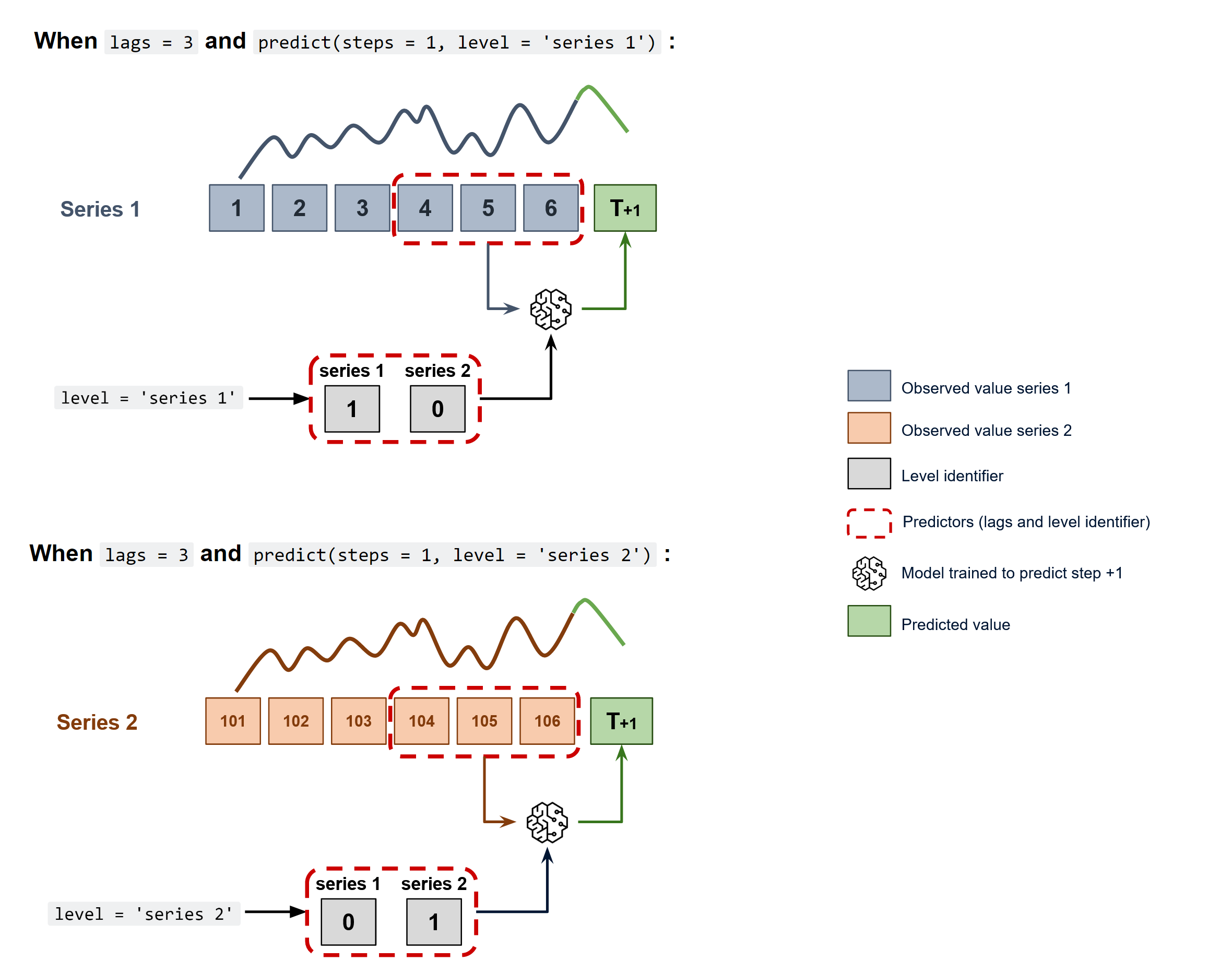
No multivariate time series

A single model is trained, but each time series remains independent of the others. In other words, the past values of one series are not used as predictors of other series. Why is it useful then to model everything together? Although the series do not depend on each other, they may follow the same intrinsic pattern regarding their past and future values. For example, in the same store, the sales of products A and B may not be related, but they follow the same dynamics, that of the store.

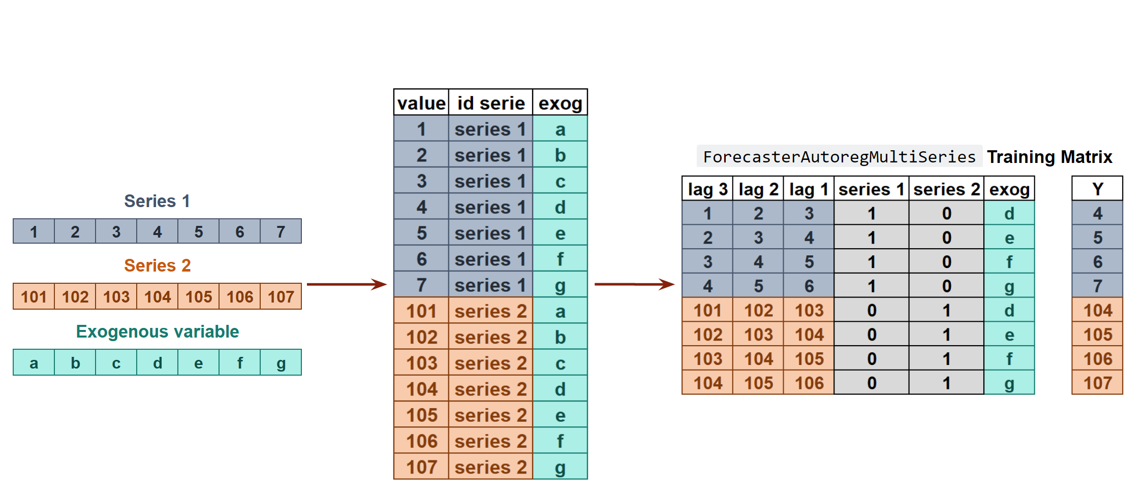
In order to predict the next n steps, the same strategy of recursive multi-step forecasting is applied. The only difference is that, the series' name for which to estimate the predictions needs to be indicated.

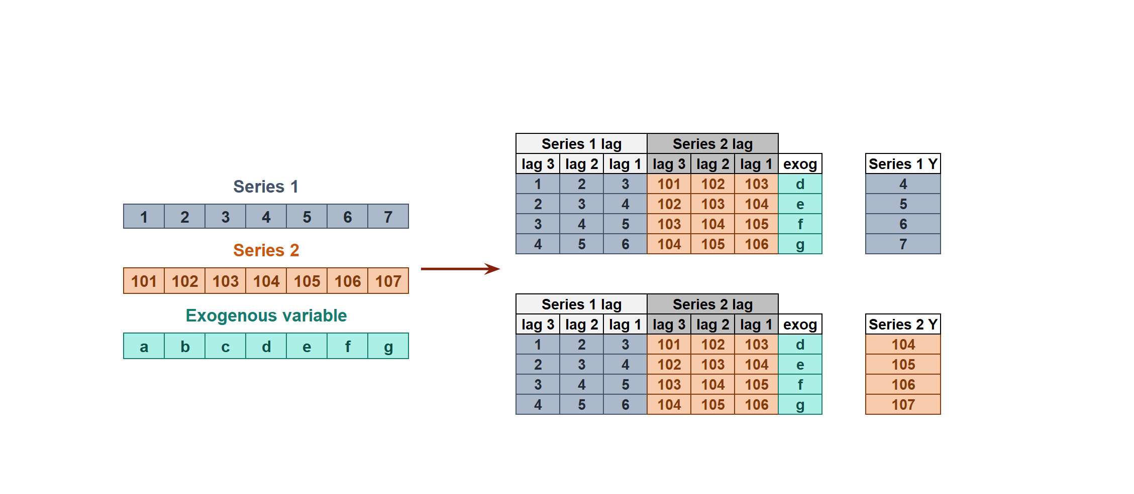
Multivariate time series

All series are modeled considering that each time series depends not only on its past values but also on the past values of the other series. The forecaster is expected not only to learn the information of each series separately but also to relate them. For example, the measurements made by all the sensors (flow, item_2, pressure...) installed on an industrial machine such as a compressor.

For a more detailed example visit: Multi-series-forecasting

  Note

ForecasterAutoregMultiSeries class covers the use case of No Multivariate time series. ForecasterAutoregMultivariate will be released in a future version of Skforecast - stay tuned!

Libraries¶

In [50]:

# Libraries
# ==============================================================================
import numpy as np
import pandas as pd
import matplotlib.pyplot as plt
from sklearn.preprocessing import StandardScaler
from sklearn.linear_model import LinearRegression
from sklearn.linear_model import Ridge
from sklearn.ensemble import RandomForestRegressor
from sklearn.metrics import mean_absolute_error

from skforecast.ForecasterAutoregMultiSeries import ForecasterAutoregMultiSeries
from skforecast.model_selection_multiseries import backtesting_forecaster_multiseries
from skforecast.model_selection_multiseries import grid_search_forecaster_multiseries

# Libraries # ============================================================================== import numpy as np import pandas as pd import matplotlib.pyplot as plt from sklearn.preprocessing import StandardScaler from sklearn.linear_model import LinearRegression from sklearn.linear_model import Ridge from sklearn.ensemble import RandomForestRegressor from sklearn.metrics import mean_absolute_error from skforecast.ForecasterAutoregMultiSeries import ForecasterAutoregMultiSeries from skforecast.model_selection_multiseries import backtesting_forecaster_multiseries from skforecast.model_selection_multiseries import grid_search_forecaster_multiseries

Data¶

In [ ]:

# Data download
# ==============================================================================
url = ('https://raw.githubusercontent.com/JoaquinAmatRodrigo/skforecast/master/' +
       'data/simulated_items_sales.csv')
data = pd.read_csv(url, sep=',')

# Data preparation (aggregation at daily level)
# ==============================================================================
data['date'] = pd.to_datetime(data['date'], format='%Y-%m-%d')
data = data.set_index('date')
data = data.asfreq('D')
data = data.sort_index()
data.head()

# Data download # ============================================================================== url = ('https://raw.githubusercontent.com/JoaquinAmatRodrigo/skforecast/master/' + 'data/simulated_items_sales.csv') data = pd.read_csv(url, sep=',') # Data preparation (aggregation at daily level) # ============================================================================== data['date'] = pd.to_datetime(data['date'], format='%Y-%m-%d') data = data.set_index('date') data = data.asfreq('D') data = data.sort_index() data.head()

In [ ]:

# Split data into train-val-test
# ==============================================================================
end_train = '2014-07-15 23:59:00'
data_train = data.loc[:end_train, :].copy()
data_test  = data.loc[end_train:, :].copy()

print(f"Train dates : {data_train.index.min()} --- {data_train.index.max()}  (n={len(data_train)})")
print(f"Test dates  : {data_test.index.min()} --- {data_test.index.max()}  (n={len(data_test)})")

# Split data into train-val-test # ============================================================================== end_train = '2014-07-15 23:59:00' data_train = data.loc[:end_train, :].copy() data_test = data.loc[end_train:, :].copy() print(f"Train dates : {data_train.index.min()} --- {data_train.index.max()} (n={len(data_train)})") print(f"Test dates : {data_test.index.min()} --- {data_test.index.max()} (n={len(data_test)})")

Train dates : 2012-01-01 00:00:00 --- 2014-07-15 00:00:00  (n=927)
Test dates  : 2014-07-16 00:00:00 --- 2015-01-01 00:00:00  (n=170)

In [ ]:

# Plot time series
# ==============================================================================
fig, axes = plt.subplots(nrows=3, ncols=1, figsize=(10, 6), sharex=True)

data_train['item_1'].plot(label='train', ax=axes[0])
data_test['item_1'].plot(label='test', ax=axes[0])
axes[0].set_xlabel('')
axes[0].set_ylabel('MW')
axes[0].set_title('Item 1')
axes[0].legend()

data_train['item_2'].plot(label='train', ax=axes[1])
data_test['item_2'].plot(label='test', ax=axes[1])
axes[1].set_xlabel('')
axes[1].set_ylabel('sales')
axes[1].set_title('Item 2')

data_train['item_3'].plot(label='train', ax=axes[2])
data_test['item_3'].plot(label='test', ax=axes[2])
axes[2].set_xlabel('')
axes[2].set_ylabel('sales')
axes[2].set_title('Item 3')

fig.tight_layout()
plt.show();

# Plot time series # ============================================================================== fig, axes = plt.subplots(nrows=3, ncols=1, figsize=(10, 6), sharex=True) data_train['item_1'].plot(label='train', ax=axes[0]) data_test['item_1'].plot(label='test', ax=axes[0]) axes[0].set_xlabel('') axes[0].set_ylabel('MW') axes[0].set_title('Item 1') axes[0].legend() data_train['item_2'].plot(label='train', ax=axes[1]) data_test['item_2'].plot(label='test', ax=axes[1]) axes[1].set_xlabel('') axes[1].set_ylabel('sales') axes[1].set_title('Item 2') data_train['item_3'].plot(label='train', ax=axes[2]) data_test['item_3'].plot(label='test', ax=axes[2]) axes[2].set_xlabel('') axes[2].set_ylabel('sales') axes[2].set_title('Item 3') fig.tight_layout() plt.show();

Train and predict ForecasterAutoregMultiSeries¶

In [ ]:

# Create and fit forecaster multi series
# ==============================================================================
forecaster = ForecasterAutoregMultiSeries(
                 regressor          = LinearRegression(),
                 lags               = 24,
                 transformer_series = None,
                 transformer_exog   = None
             )

forecaster.fit(series=data_train)
forecaster

# Create and fit forecaster multi series # ============================================================================== forecaster = ForecasterAutoregMultiSeries( regressor = LinearRegression(), lags = 24, transformer_series = None, transformer_exog = None ) forecaster.fit(series=data_train) forecaster

Out[ ]:

============================ 
ForecasterAutoregMultiSeries 
============================ 
Regressor: LinearRegression() 
Lags: [ 1  2  3  4  5  6  7  8  9 10 11 12 13 14 15 16 17 18 19 20 21 22 23 24] 
Transformer for series: {'item_1': None, 'item_2': None, 'item_3': None} 
Transformer for exog: None 
Window size: 24 
Series levels: ['item_1', 'item_2', 'item_3'] 
Included exogenous: False 
Type of exogenous variable: None 
Exogenous variables names: None 
Training range: [Timestamp('2012-01-01 00:00:00'), Timestamp('2014-07-15 00:00:00')] 
Training index type: DatetimeIndex 
Training index frequency: D 
Regressor parameters: {'copy_X': True, 'fit_intercept': True, 'n_jobs': None, 'normalize': 'deprecated', 'positive': False} 
Creation date: 2022-10-13 16:46:31 
Last fit date: 2022-10-13 16:46:32 
Skforecast version: 0.5.1 
Python version: 3.9.13 

Two methods can be use to predict the next n steps: predict() or predict_interval(). The argument level is used to indicate for which series estimate predictions.

In [ ]:

# Predict and predict_interval
# ==============================================================================
steps = 24

# Predictions for item_1
predictions_item_1 = forecaster.predict(steps=steps, level='item_1')
display(predictions_item_1.head(3))

# Interval predictions for item_1
predictions_temp = forecaster.predict_interval(steps=steps, level='item_1')
display(predictions_temp.head(3))

# Predict and predict_interval # ============================================================================== steps = 24 # Predictions for item_1 predictions_item_1 = forecaster.predict(steps=steps, level='item_1') display(predictions_item_1.head(3)) # Interval predictions for item_1 predictions_temp = forecaster.predict_interval(steps=steps, level='item_1') display(predictions_temp.head(3))

2014-07-16    25.497655
2014-07-17    24.867333
2014-07-18    24.281557
Freq: D, Name: pred, dtype: float64

	pred	lower_bound	upper_bound
2014-07-16	25.497655	23.220017	28.226023
2014-07-17	24.867333	22.141024	27.389717
2014-07-18	24.281557	21.688227	26.981138

Backtesting Multi Series¶

As in the predict method, the level at which backtesting is performed must be indicated.

In [ ]:

# Backtesting Multi Series
# ==============================================================================
metric, predictions_item_1 = backtesting_forecaster_multiseries(
                                 forecaster         = forecaster,
                                 series             = data,
                                 level              = 'item_1',
                                 initial_train_size = len(data_train),
                                 fixed_train_size   = True,
                                 steps              = 24,
                                 metric             = 'mean_absolute_error',
                                 refit              = True,
                                 verbose            = False
                             )

print(f"Backtest error item_1: {metric}")
predictions_item_1.head(4)

# Backtesting Multi Series # ============================================================================== metric, predictions_item_1 = backtesting_forecaster_multiseries( forecaster = forecaster, series = data, level = 'item_1', initial_train_size = len(data_train), fixed_train_size = True, steps = 24, metric = 'mean_absolute_error', refit = True, verbose = False ) print(f"Backtest error item_1: {metric}") predictions_item_1.head(4)

Backtest error item_1: 1.3607708085816819

Out[ ]:

	pred
2014-07-16	25.497655
2014-07-17	24.867333
2014-07-18	24.281557
2014-07-19	23.515885

Hyperparameter tuning and lags selection Multi Series¶

Functions grid_search_forecaster_multiseries and random_search_forecaster_multiseries in the module model_selection_multiseries allow for lag and hyperparameter optimization. The optimization is performed in the same way as in the other forecasters, see the user guide here, except for two arguments:

• levels: level(s) at which the forecaster is optimized, for example:

  • If levels = ['item_1', 'item_2'] (Same as levels = None), the function will search for the lags and hyperparameters that minimize the average error of the predictions of both time series. The resulting metric will be a weighted average of the optimization of both levels.

  • If levels = 'item_1' (Same as levels = ['item_1']), the function will search for the lags and hyperparameters that minimize the error of the item_1 predictions.

• levels_weights: weights given to each level during optimization, for example:

  • If levels = ['item_1', 'item_2'] and levels_weights = {'item_1': 0.5, 'item_2': 0.5} (Same as levels_weights = None), both time series will have the same weight in the calculation of the resulting metric.

The following example shows how to use grid_search_forecaster_multiseries to find the best lags and model hyperparameters for both time series:

In [ ]:

# Create and fit forecaster multi series
# ==============================================================================
forecaster = ForecasterAutoregMultiSeries(
                 regressor          = Ridge(random_state=123),
                 lags               = 24,
                 transformer_series = StandardScaler(),
                 transformer_exog   = None
             )

# Create and fit forecaster multi series # ============================================================================== forecaster = ForecasterAutoregMultiSeries( regressor = Ridge(random_state=123), lags = 24, transformer_series = StandardScaler(), transformer_exog = None )

In [ ]:

# Grid search Multi Series
# ==============================================================================
lags_grid = [24, 48]
param_grid = {'alpha': [0.01, 0.1, 1]}

levels = ['item_1', 'item_2', 'item_3']

results = grid_search_forecaster_multiseries(
              forecaster          = forecaster,
              series              = data,
              lags_grid           = lags_grid,
              param_grid          = param_grid,
              steps               = 24,
              metric              = 'mean_absolute_error',
              initial_train_size  = len(data_train),
              fixed_train_size    = True,
              levels              = levels,
              exog                = None,
              refit               = True,
              return_best         = False,
              verbose             = False
          )

results

# Grid search Multi Series # ============================================================================== lags_grid = [24, 48] param_grid = {'alpha': [0.01, 0.1, 1]} levels = ['item_1', 'item_2', 'item_3'] results = grid_search_forecaster_multiseries( forecaster = forecaster, series = data, lags_grid = lags_grid, param_grid = param_grid, steps = 24, metric = 'mean_absolute_error', initial_train_size = len(data_train), fixed_train_size = True, levels = levels, exog = None, refit = True, return_best = False, verbose = False ) results

6 models compared for 3 level(s). Number of iterations: 18.
Level weights for metric evaluation: {'item_1': 0.3333333333333333, 'item_2': 0.3333333333333333, 'item_3': 0.3333333333333333}

loop lags_grid: 100%|███████████████████████████████████████| 2/2 [00:08<00:00,  4.04s/it]

Out[ ]:

	levels	lags	params	mean_absolute_error	alpha
5	[item_1, item_2, item_3]	[1, 2, 3, 4, 5, 6, 7, 8, 9, 10, 11, 12, 13, 14...	{'alpha': 1}	2.207648	1.00
4	[item_1, item_2, item_3]	[1, 2, 3, 4, 5, 6, 7, 8, 9, 10, 11, 12, 13, 14...	{'alpha': 0.1}	2.207700	0.10
3	[item_1, item_2, item_3]	[1, 2, 3, 4, 5, 6, 7, 8, 9, 10, 11, 12, 13, 14...	{'alpha': 0.01}	2.207706	0.01
2	[item_1, item_2, item_3]	[1, 2, 3, 4, 5, 6, 7, 8, 9, 10, 11, 12, 13, 14...	{'alpha': 1}	2.335039	1.00
1	[item_1, item_2, item_3]	[1, 2, 3, 4, 5, 6, 7, 8, 9, 10, 11, 12, 13, 14...	{'alpha': 0.1}	2.335149	0.10
0	[item_1, item_2, item_3]	[1, 2, 3, 4, 5, 6, 7, 8, 9, 10, 11, 12, 13, 14...	{'alpha': 0.01}	2.335161	0.01

  Warning

Use multiple metrics in the hyperparameter tuning and bayesian_search_forecaster_multiseries will be released in a future version of Skforecast Stay tuned!

In [ ]:

%%html
<style>
.jupyter-wrapper .jp-CodeCell .jp-Cell-inputWrapper .jp-InputPrompt {display: none;}
</style>

%%html