Recursive multi-step forecasting¶

Since the value of $t_{n-1}$ is required to predict $t_n$, and $t_{n-1}$ is unknown, a recursive process is applied in which, each new prediction, is based on the previous one. This process is known as recursive forecasting or recursive multi-step forecasting.

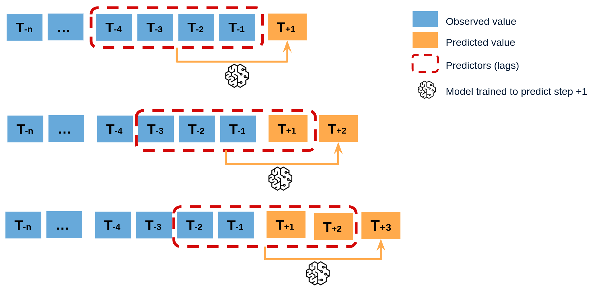
The major challenge when using machine learning models for recursive multi-step forecasting is transforming the time series into a matrix where each value of the series is related to the time window (lags) that precedes it. This forecasting strategy can be easily generated with the classes ForecasterAutoreg and ForecasterAutoregCustom.

Libraries¶

In [1]:

# Libraries
# ==============================================================================
import pandas as pd
import matplotlib.pyplot as plt
from skforecast.ForecasterAutoreg import ForecasterAutoreg
from sklearn.ensemble import RandomForestRegressor
from sklearn.metrics import mean_squared_error

# Libraries # ============================================================================== import pandas as pd import matplotlib.pyplot as plt from skforecast.ForecasterAutoreg import ForecasterAutoreg from sklearn.ensemble import RandomForestRegressor from sklearn.metrics import mean_squared_error

Data¶

In [2]:

# Download data
# ==============================================================================
url = ('https://raw.githubusercontent.com/JoaquinAmatRodrigo/skforecast/master/data/h2o.csv')
data = pd.read_csv(url, sep=',', header=0, names=['y', 'datetime'])

# Data preprocessing
# ==============================================================================
data['datetime'] = pd.to_datetime(data['datetime'], format='%Y/%m/%d')
data = data.set_index('datetime')
data = data.asfreq('MS')
data = data['y']
data = data.sort_index()

# Split train-test
# ==============================================================================
steps = 36
data_train = data[:-steps]
data_test  = data[-steps:]

# Plot
# ==============================================================================
fig, ax=plt.subplots(figsize=(9, 4))
data_train.plot(ax=ax, label='train')
data_test.plot(ax=ax, label='test')
ax.legend();

# Download data # ============================================================================== url = ('https://raw.githubusercontent.com/JoaquinAmatRodrigo/skforecast/master/data/h2o.csv') data = pd.read_csv(url, sep=',', header=0, names=['y', 'datetime']) # Data preprocessing # ============================================================================== data['datetime'] = pd.to_datetime(data['datetime'], format='%Y/%m/%d') data = data.set_index('datetime') data = data.asfreq('MS') data = data['y'] data = data.sort_index() # Split train-test # ============================================================================== steps = 36 data_train = data[:-steps] data_test = data[-steps:] # Plot # ============================================================================== fig, ax=plt.subplots(figsize=(9, 4)) data_train.plot(ax=ax, label='train') data_test.plot(ax=ax, label='test') ax.legend();

Train forecaster¶

In [3]:

# Create and fit forecaster
# ==============================================================================
forecaster = ForecasterAutoreg(
                 regressor = RandomForestRegressor(random_state=123),
                 lags      = 15
             )

forecaster.fit(y=data_train)
forecaster

# Create and fit forecaster # ============================================================================== forecaster = ForecasterAutoreg( regressor = RandomForestRegressor(random_state=123), lags = 15 ) forecaster.fit(y=data_train) forecaster

Out[3]:

================= 
ForecasterAutoreg 
================= 
Regressor: RandomForestRegressor(random_state=123) 
Lags: [ 1  2  3  4  5  6  7  8  9 10 11 12 13 14 15] 
Transformer for y: None 
Transformer for exog: None 
Window size: 15 
Included exogenous: False 
Type of exogenous variable: None 
Exogenous variables names: None 
Training range: [Timestamp('1991-07-01 00:00:00'), Timestamp('2005-06-01 00:00:00')] 
Training index type: DatetimeIndex 
Training index frequency: MS 
Regressor parameters: {'bootstrap': True, 'ccp_alpha': 0.0, 'criterion': 'squared_error', 'max_depth': None, 'max_features': 1.0, 'max_leaf_nodes': None, 'max_samples': None, 'min_impurity_decrease': 0.0, 'min_samples_leaf': 1, 'min_samples_split': 2, 'min_weight_fraction_leaf': 0.0, 'n_estimators': 100, 'n_jobs': None, 'oob_score': False, 'random_state': 123, 'verbose': 0, 'warm_start': False} 
Creation date: 2022-09-24 08:20:30 
Last fit date: 2022-09-24 08:20:30 
Skforecast version: 0.5.0 
Python version: 3.9.13 

Prediction¶

In [4]:

# Predict
# ==============================================================================
predictions = forecaster.predict(steps=36)
predictions.head(3)

# Predict # ============================================================================== predictions = forecaster.predict(steps=36) predictions.head(3)

Out[4]:

2005-07-01    0.921840
2005-08-01    0.954921
2005-09-01    1.101716
Freq: MS, Name: pred, dtype: float64

In [5]:

# Plot predictions
# ==============================================================================
fig, ax=plt.subplots(figsize=(9, 4))
data_train.plot(ax=ax, label='train')
data_test.plot(ax=ax, label='test')
predictions.plot(ax=ax, label='predictions')
ax.legend();

# Plot predictions # ============================================================================== fig, ax=plt.subplots(figsize=(9, 4)) data_train.plot(ax=ax, label='train') data_test.plot(ax=ax, label='test') predictions.plot(ax=ax, label='predictions') ax.legend();

In [6]:

# Prediction error
# ==============================================================================
error_mse = mean_squared_error(
                y_true = data_test,
                y_pred = predictions
            )
print(f"Test error (mse): {error_mse}")

# Prediction error # ============================================================================== error_mse = mean_squared_error( y_true = data_test, y_pred = predictions ) print(f"Test error (mse): {error_mse}")

Test error (mse): 0.00429855684785846

Prediction intervals¶

A prediction interval defines the interval within which the true value of y is expected to be found with a given probability. For example, the prediction interval (1, 99) can be expected to contain the true prediction value with 98% probability.

By default, every ForecasterAutoreg and ForecasterAutoregCustom can estimate prediction intervals using the method predict_interval. For a detailed explanation of the different prediction intervals available in skforecast visit Prediction intervals.

In [7]:

# Predict intervals
# ==============================================================================
predictions = forecaster.predict_interval(steps=36, interval=[5, 95], n_boot=100)
predictions.head(3)

# Predict intervals # ============================================================================== predictions = forecaster.predict_interval(steps=36, interval=[5, 95], n_boot=100) predictions.head(3)

Out[7]:

	pred	lower_bound	upper_bound
2005-07-01	0.921840	0.884362	0.960898
2005-08-01	0.954921	0.923163	0.980901
2005-09-01	1.101716	1.057791	1.143083

Feature importance¶

In [8]:

forecaster.get_feature_importance()

forecaster.get_feature_importance()

Out[8]:

	feature	importance
0	lag_1	0.012340
1	lag_2	0.085160
2	lag_3	0.013407
3	lag_4	0.004374
4	lag_5	0.003188
5	lag_6	0.003436
6	lag_7	0.003136
7	lag_8	0.007141
8	lag_9	0.007831
9	lag_10	0.012751
10	lag_11	0.009019
11	lag_12	0.807098
12	lag_13	0.004811
13	lag_14	0.016328
14	lag_15	0.009979

Extract training matrix¶

In [9]:

X, y = forecaster.create_train_X_y(data_train)
X.head()

X, y = forecaster.create_train_X_y(data_train) X.head()

Out[9]:

	lag_1	lag_2	lag_3	lag_4	lag_5	lag_6	lag_7	lag_8	lag_9	lag_10	lag_11	lag_12	lag_13	lag_14	lag_15
datetime
1992-10-01	0.534761	0.475463	0.483389	0.410534	0.361801	0.379808	0.351348	0.336220	0.660119	0.602652	0.502369	0.492543	0.432159	0.400906	0.429795
1992-11-01	0.568606	0.534761	0.475463	0.483389	0.410534	0.361801	0.379808	0.351348	0.336220	0.660119	0.602652	0.502369	0.492543	0.432159	0.400906
1992-12-01	0.595223	0.568606	0.534761	0.475463	0.483389	0.410534	0.361801	0.379808	0.351348	0.336220	0.660119	0.602652	0.502369	0.492543	0.432159
1993-01-01	0.771258	0.595223	0.568606	0.534761	0.475463	0.483389	0.410534	0.361801	0.379808	0.351348	0.336220	0.660119	0.602652	0.502369	0.492543
1993-02-01	0.751503	0.771258	0.595223	0.568606	0.534761	0.475463	0.483389	0.410534	0.361801	0.379808	0.351348	0.336220	0.660119	0.602652	0.502369

In [10]:

y.head()

y.head()

Out[10]:

datetime
1992-10-01    0.568606
1992-11-01    0.595223
1992-12-01    0.771258
1993-01-01    0.751503
1993-02-01    0.387554
Freq: MS, Name: y, dtype: float64

In [11]:

%%html
<style>
.jupyter-wrapper .jp-CodeCell .jp-Cell-inputWrapper .jp-InputPrompt {display: none;}
</style>

%%html