Backtesting
Backtesting is a term used in modeling to refer to testing a predictive model on historical data. Backtesting involves moving backward in time, step-by-step, in as many stages as is necessary. Therefore, it is a special type of cross-validation applied to previous period(s).
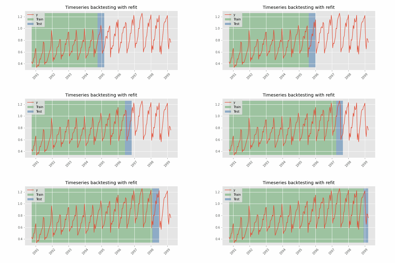
Backtesting with refit and increasing training size (fixed origin)
The model is trained each time before making predictions. With this configuration, the model uses all the data available so far. It is a variation of the standard cross-validation but, instead of making a random distribution of the observations, the training set increases sequentially, maintaining the temporal order of the data.


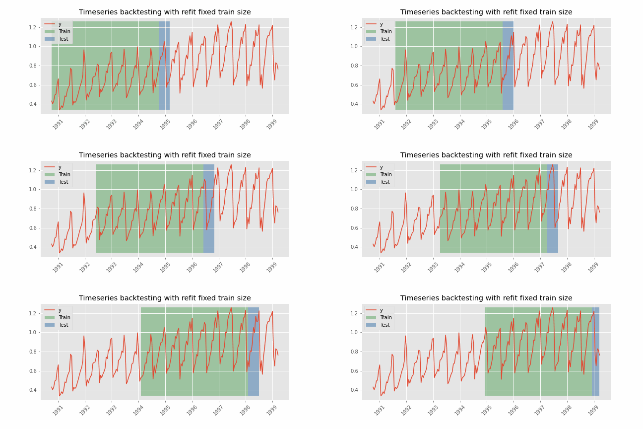
Backtesting with refit and fixed training size (rolling origin)
A technique similar to the previous one but, in this case, the forecast origin rolls forward, therefore, the size of training remains constant. This is also known as time series cross-validation or walk-forward validation.


Backtesting without refit
After an initial train, the model is used sequentially without updating it and following the temporal order of the data. This strategy has the advantage of being much faster since the model is trained only once. However, the model does not incorporate the latest information available, so it may lose predictive capacity over time.


Libraries
# Libraries
# ==============================================================================
import numpy as np
import pandas as pd
import matplotlib.pyplot as plt
from skforecast.ForecasterAutoreg import ForecasterAutoreg
from skforecast.model_selection import backtesting_forecaster
from sklearn.linear_model import Ridge
from sklearn.ensemble import RandomForestRegressor
from sklearn.metrics import mean_squared_error
Data
# Download data
# ==============================================================================
url = ('https://raw.githubusercontent.com/JoaquinAmatRodrigo/skforecast/master/data/h2o.csv')
data = pd.read_csv(url, sep=',', header=0, names=['y', 'datetime'])

# Data preprocessing
# ==============================================================================
data['datetime'] = pd.to_datetime(data['datetime'], format='%Y/%m/%d')
data = data.set_index('datetime')
data = data.asfreq('MS')
data = data[['y']]
data = data.sort_index()

# Train-validation dates
# ==============================================================================
end_train = '2002-01-01 23:59:00'

print(f"Train dates      : {data.index.min()} --- {data.loc[:end_train].index.max()}  (n={len(data.loc[:end_train])})")
print(f"Validation dates : {data.loc[end_train:].index.min()} --- {data.index.max()}  (n={len(data.loc[end_train:])})")

# Plot
# ==============================================================================
fig, ax=plt.subplots(figsize=(9, 4))
data.loc[:end_train].plot(ax=ax, label='train')
data.loc[end_train:].plot(ax=ax, label='validation')
ax.legend()
plt.show()

display(data.head(4))
Train dates      : 1991-07-01 00:00:00 --- 2002-01-01 00:00:00  (n=127)
Validation dates : 2002-02-01 00:00:00 --- 2008-06-01 00:00:00  (n=77)
| y | |
|---|---|
| datetime | |
| 1991-07-01 | 0.429795 |
| 1991-08-01 | 0.400906 |
| 1991-09-01 | 0.432159 |
| 1991-10-01 | 0.492543 |
Backtest
The backtesting process adapted to this scenario is:
The model is trained with the series length set in
initial_train_size.It predicts and stores the next 10 steps,
steps=10.Since
refit=True, the training set increases to a length ofinitial_train_size+steps, and the test data becomes the following 10 steps.The model is re-trained with the new training set. The new 10 steps are then predicted.
This process is repeated until the entire series has been run.
# Backtest forecaster
# ==============================================================================
forecaster = ForecasterAutoreg(
                 regressor = RandomForestRegressor(random_state=123),
                 lags      = 15
             )

metric, predictions_backtest = backtesting_forecaster(
                                   forecaster         = forecaster,
                                   y                  = data['y'],
                                   initial_train_size = len(data.loc[:end_train]),
                                   fixed_train_size   = False,
                                   steps              = 10,
                                   metric             = 'mean_squared_error',
                                   refit              = True,
                                   verbose            = True
                               )
Information of backtesting process
----------------------------------
Number of observations used for initial training: 127
Number of observations used for backtesting: 77
    Number of folds: 8
    Number of steps per fold: 10
    Last fold only includes 7 observations.

Data partition in fold: 0
    Training:   1991-07-01 00:00:00 -- 2002-01-01 00:00:00  (n=127)
    Validation: 2002-02-01 00:00:00 -- 2002-11-01 00:00:00  (n=10)
Data partition in fold: 1
    Training:   1991-07-01 00:00:00 -- 2002-11-01 00:00:00  (n=137)
    Validation: 2002-12-01 00:00:00 -- 2003-09-01 00:00:00  (n=10)
Data partition in fold: 2
    Training:   1991-07-01 00:00:00 -- 2003-09-01 00:00:00  (n=147)
    Validation: 2003-10-01 00:00:00 -- 2004-07-01 00:00:00  (n=10)
Data partition in fold: 3
    Training:   1991-07-01 00:00:00 -- 2004-07-01 00:00:00  (n=157)
    Validation: 2004-08-01 00:00:00 -- 2005-05-01 00:00:00  (n=10)
Data partition in fold: 4
    Training:   1991-07-01 00:00:00 -- 2005-05-01 00:00:00  (n=167)
    Validation: 2005-06-01 00:00:00 -- 2006-03-01 00:00:00  (n=10)
Data partition in fold: 5
    Training:   1991-07-01 00:00:00 -- 2006-03-01 00:00:00  (n=177)
    Validation: 2006-04-01 00:00:00 -- 2007-01-01 00:00:00  (n=10)
Data partition in fold: 6
    Training:   1991-07-01 00:00:00 -- 2007-01-01 00:00:00  (n=187)
    Validation: 2007-02-01 00:00:00 -- 2007-11-01 00:00:00  (n=10)
Data partition in fold: 7
    Training:   1991-07-01 00:00:00 -- 2007-11-01 00:00:00  (n=197)
    Validation: 2007-12-01 00:00:00 -- 2008-06-01 00:00:00  (n=7)
print(f"Backtest error: {metric}")
Backtest error: 0.00818535931502708
predictions_backtest.head(4)
| pred | |
|---|---|
| 2002-02-01 | 0.594506 |
| 2002-03-01 | 0.785886 |
| 2002-04-01 | 0.698925 |
| 2002-05-01 | 0.790560 |
fig, ax = plt.subplots(figsize=(9, 4))
data.loc[end_train:, 'y'].plot(ax=ax)
predictions_backtest.plot(ax=ax)
ax.legend();
Backtest with prediction intervals
# Backtest forecaster
# ==============================================================================
forecaster = ForecasterAutoreg(
                 regressor = Ridge(),
                 lags      = 15
             )

metric, predictions_backtest = backtesting_forecaster(
                                   forecaster         = forecaster,
                                   y                  = data['y'],
                                   initial_train_size = len(data.loc[:end_train]),
                                   fixed_train_size   = False,
                                   steps              = 10,
                                   metric             = 'mean_squared_error',
                                   refit              = True,
                                   interval           = [5, 95],
                                   n_boot             = 500,
                                   verbose            = True
                               )
Information of backtesting process
----------------------------------
Number of observations used for initial training: 127
Number of observations used for backtesting: 77
    Number of folds: 8
    Number of steps per fold: 10
    Last fold only includes 7 observations.

Data partition in fold: 0
    Training:   1991-07-01 00:00:00 -- 2002-01-01 00:00:00  (n=127)
    Validation: 2002-02-01 00:00:00 -- 2002-11-01 00:00:00  (n=10)
Data partition in fold: 1
    Training:   1991-07-01 00:00:00 -- 2002-11-01 00:00:00  (n=137)
    Validation: 2002-12-01 00:00:00 -- 2003-09-01 00:00:00  (n=10)
Data partition in fold: 2
    Training:   1991-07-01 00:00:00 -- 2003-09-01 00:00:00  (n=147)
    Validation: 2003-10-01 00:00:00 -- 2004-07-01 00:00:00  (n=10)
Data partition in fold: 3
    Training:   1991-07-01 00:00:00 -- 2004-07-01 00:00:00  (n=157)
    Validation: 2004-08-01 00:00:00 -- 2005-05-01 00:00:00  (n=10)
Data partition in fold: 4
    Training:   1991-07-01 00:00:00 -- 2005-05-01 00:00:00  (n=167)
    Validation: 2005-06-01 00:00:00 -- 2006-03-01 00:00:00  (n=10)
Data partition in fold: 5
    Training:   1991-07-01 00:00:00 -- 2006-03-01 00:00:00  (n=177)
    Validation: 2006-04-01 00:00:00 -- 2007-01-01 00:00:00  (n=10)
Data partition in fold: 6
    Training:   1991-07-01 00:00:00 -- 2007-01-01 00:00:00  (n=187)
    Validation: 2007-02-01 00:00:00 -- 2007-11-01 00:00:00  (n=10)
Data partition in fold: 7
    Training:   1991-07-01 00:00:00 -- 2007-11-01 00:00:00  (n=197)
    Validation: 2007-12-01 00:00:00 -- 2008-06-01 00:00:00  (n=7)
predictions_backtest.head()
| pred | lower_bound | upper_bound | |
|---|---|---|---|
| 2002-02-01 | 0.703579 | 0.599636 | 0.834616 |
| 2002-03-01 | 0.673522 | 0.572605 | 0.787942 |
| 2002-04-01 | 0.698319 | 0.589196 | 0.815748 |
| 2002-05-01 | 0.703042 | 0.593719 | 0.831795 |
| 2002-06-01 | 0.733776 | 0.632476 | 0.842865 |
fig, ax=plt.subplots(figsize=(9, 4))
data.loc[end_train:, 'y'].plot(ax=ax, label='test')
predictions_backtest['pred'].plot(ax=ax, label='predictions')
ax.fill_between(
    predictions_backtest.index,
    predictions_backtest['lower_bound'],
    predictions_backtest['upper_bound'],
    color = 'red',
    alpha = 0.2,
    label = 'prediction interval'
)
ax.legend();
# Fit forecaster
# ==============================================================================
forecaster = ForecasterAutoreg(
                 regressor = RandomForestRegressor(random_state=123),
                 lags      = 15
             )

forecaster.fit(y=data['y'])
Set arguments initial_train_size=None and refit=False to perform backtesting using the already trained forecaster.
# Backtest train data
# ==============================================================================
metric, predictions_train = backtesting_forecaster(
                                forecaster         = forecaster,
                                y                  = data['y'],
                                initial_train_size = None,
                                steps              = 1,
                                metric             = 'mean_squared_error',
                                refit              = False,
                                verbose            = False
                            )

print(f"Backtest training error: {metric}")
Backtest training error: 0.0005392479040738611
predictions_train.head(4)
| pred | |
|---|---|
| 1992-10-01 | 0.553611 |
| 1992-11-01 | 0.568324 |
| 1992-12-01 | 0.735167 |
| 1993-01-01 | 0.723217 |
The first 15 observations are not predicted since they are needed to create the lags used as predictors.
# Plot training predictions
# ==============================================================================
fig, ax = plt.subplots(figsize=(9, 4))
data.plot(ax=ax)
predictions_train.plot(ax=ax)
ax.legend();
Predict using the internal regressor
# Fit forecaster
# ==============================================================================
forecaster = ForecasterAutoreg(
                 regressor = RandomForestRegressor(random_state=123),
                 lags      = 15
             )

forecaster.fit(y=data['y'])
# Create training matrix
# ==============================================================================
X, y = forecaster.create_train_X_y(
           y = data['y'],
           exog = None
       )
Using the internal regressor only allows predicting one step ahead.
# Predict using the internal regressor
# ==============================================================================
forecaster.regressor.predict(X)[:4]
array([0.55361079, 0.56832448, 0.73516725, 0.72321715])
Backtest with custom metric
Besides the frequently used metrics: mean_squared_error, mean_absolute_error, and mean_absolute_percentage_error, it is possible to use any custom function as long as:
It includes the arguments:
y_true: true values of the series.y_pred: predicted values.
It returns a numeric value (
floatorint).
It allows evaluating the predictive capability of the model in a wide range of scenarios, for example:
Consider only certain months, days, hours...
Consider only dates that are holidays.
Consider only the last step of the predicted horizon.
The following example shows how to forecast a 12-month horizon but considering only the last 3 months of each year to calculate the interest metric.
# Backtest forecaster with custom metric
# ==============================================================================
def custom_metric(y_true, y_pred):
    """
    Calculate the mean squared error using only the predicted values of the last
    3 months of the year.
    """
    mask = y_true.index.month.isin([10, 11, 12])
    metric = mean_squared_error(y_true[mask], y_pred[mask])

    return metric

metric, predictions_backtest = backtesting_forecaster(
                                   forecaster         = forecaster,
                                   y                  = data['y'],
                                   initial_train_size = len(data.loc[:end_train]),
                                   fixed_train_size   = False,
                                   steps              = 10,
                                   metric             = custom_metric,
                                   refit              = True,
                                   verbose            = False
                               )

print(f"Backtest error custom metric: {metric}")
Backtest error custom metric: 0.005580948738772139
Backtest with multiple metrics
The function backtesting_forecaster allow to estimate multiple metrics at the same time if a list of metrics is provided. This list may include custom metrics.
metrics, predictions_backtest = backtesting_forecaster(
                                    forecaster         = forecaster,
                                    y                  = data['y'],
                                    initial_train_size = len(data.loc[:end_train]),
                                    fixed_train_size   = False,
                                    steps              = 10,
                                    metric             = ['mean_squared_error', 'mean_absolute_error'],
                                    refit              = True,
                                    verbose            = False
                                )

print(f"Backtest error metrics: {metrics}")
Backtest error metrics: [0.00818535931502708, 0.06489120319220776]
Backtest with exogenous variables
# Download data
# ==============================================================================
url = ('https://raw.githubusercontent.com/JoaquinAmatRodrigo/skforecast/master/data/h2o_exog.csv')
data = pd.read_csv(url, sep=',', header=0, names=['datetime', 'y', 'exog_1', 'exog_2'])

# Data preprocessing
# ==============================================================================
data['datetime'] = pd.to_datetime(data['datetime'], format='%Y/%m/%d')
data = data.set_index('datetime')
data = data.asfreq('MS')
data = data.sort_index()

# Train-validation dates
# ==============================================================================
end_train = '2002-01-01 23:59:00'

print(f"Train dates      : {data.index.min()} --- {data.loc[:end_train].index.max()}  (n={len(data.loc[:end_train])})")
print(f"Validation dates : {data.loc[end_train:].index.min()} --- {data.index.max()}  (n={len(data.loc[end_train:])})")

# Plot
# ==============================================================================
fig, ax=plt.subplots(figsize=(9, 4))
data.plot(ax=ax);
Train dates      : 1992-04-01 00:00:00 --- 2002-01-01 00:00:00  (n=118)
Validation dates : 2002-02-01 00:00:00 --- 2008-06-01 00:00:00  (n=77)
# Backtest forecaster exogenous variables
# ==============================================================================
forecaster = ForecasterAutoreg(
                 regressor = RandomForestRegressor(random_state=123),
                 lags      = 15
             )

metric, predictions_backtest = backtesting_forecaster(
                                   forecaster = forecaster,
                                   y          = data['y'],
                                   exog       = data[['exog_1', 'exog_2']],
                                   initial_train_size = len(data.loc[:end_train]),
                                   fixed_train_size   = False,
                                   steps      = 10,
                                   metric     = 'mean_squared_error',
                                   refit      = True,
                                   verbose    = True
                               )
Information of backtesting process
----------------------------------
Number of observations used for initial training: 118
Number of observations used for backtesting: 77
    Number of folds: 8
    Number of steps per fold: 10
    Last fold only includes 7 observations.

Data partition in fold: 0
    Training:   1992-04-01 00:00:00 -- 2002-01-01 00:00:00  (n=118)
    Validation: 2002-02-01 00:00:00 -- 2002-11-01 00:00:00  (n=10)
Data partition in fold: 1
    Training:   1992-04-01 00:00:00 -- 2002-11-01 00:00:00  (n=128)
    Validation: 2002-12-01 00:00:00 -- 2003-09-01 00:00:00  (n=10)
Data partition in fold: 2
    Training:   1992-04-01 00:00:00 -- 2003-09-01 00:00:00  (n=138)
    Validation: 2003-10-01 00:00:00 -- 2004-07-01 00:00:00  (n=10)
Data partition in fold: 3
    Training:   1992-04-01 00:00:00 -- 2004-07-01 00:00:00  (n=148)
    Validation: 2004-08-01 00:00:00 -- 2005-05-01 00:00:00  (n=10)
Data partition in fold: 4
    Training:   1992-04-01 00:00:00 -- 2005-05-01 00:00:00  (n=158)
    Validation: 2005-06-01 00:00:00 -- 2006-03-01 00:00:00  (n=10)
Data partition in fold: 5
    Training:   1992-04-01 00:00:00 -- 2006-03-01 00:00:00  (n=168)
    Validation: 2006-04-01 00:00:00 -- 2007-01-01 00:00:00  (n=10)
Data partition in fold: 6
    Training:   1992-04-01 00:00:00 -- 2007-01-01 00:00:00  (n=178)
    Validation: 2007-02-01 00:00:00 -- 2007-11-01 00:00:00  (n=10)
Data partition in fold: 7
    Training:   1992-04-01 00:00:00 -- 2007-11-01 00:00:00  (n=188)
    Validation: 2007-12-01 00:00:00 -- 2008-06-01 00:00:00  (n=7)
print(f"Backtest error with exogenous variables: {metric}")
Backtest error with exogenous variables: 0.007800037462113706
fig, ax = plt.subplots(figsize=(9, 4))
data.loc[end_train:].plot(ax=ax)
predictions_backtest.plot(ax=ax)
ax.legend();
%%html
<style>
.jupyter-wrapper .jp-CodeCell .jp-Cell-inputWrapper .jp-InputPrompt {display: none;}
</style>