Probabilistic Forecasting: Conformal Prediction
Conformal prediction is a framework for constructing prediction intervals that are guaranteed to contain the true value with a specified probability (coverage probability), under the assumption that the data are exchangeable. It works by combining the predictions of a point-forecasting model with its past residuals (differences between the actual values and the predictions). These residuals help estimate the uncertainty in the forecast and determine the margin that is added to and subtracted from the point forecast to build the interval. Skforecast implements Split Conformal Prediction (SCP).
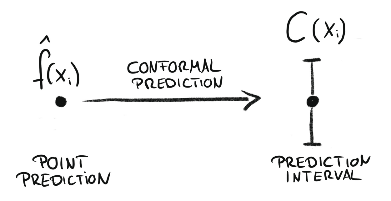
Conformal regression turns point predictions into prediction intervals. Source: Introduction To Conformal Prediction With Python: A Short Guide For Quantifying Uncertainty Of Machine Learning Models
by Christoph Molnar, leanpub.com/conformal-prediction
Conformal methods can also calibrate prediction intervals generated by other techniques, such as quantile regression or bootstrapped residuals. In this case, the conformal method adjusts the prediction intervals to bring their empirical coverage closer to the nominal coverage. Skforecast provides this functionality through the ConformalIntervalCalibrator transformer, as shown in the conformal calibration user guide.
⚠ Warning
The coverage guarantee of conformal prediction relies on the exchangeability of the data, an assumption that time series do not satisfy because of autocorrelation, trends, seasonality and changes in their dynamics. In addition, in multi-step-ahead forecasting the errors usually grow with the horizon, while a single correction factor is applied to all the steps. For these reasons, the nominal coverage is only approximate in forecasting, and the empirical coverage should always be validated with backtesting.
There are several well-established methods for conformal prediction, each with its own characteristics and assumptions. Skforecast implements Split Conformal Prediction due to its balance between simplicity and performance.
💡 Tip
For more examples on how to use probabilistic forecasting, check out the following articles:
How split conformal prediction works
Given a nominal coverage (for example, for an 80% interval), split conformal prediction builds the interval in three steps:
Calibration residuals. The model predicts a set of observations that were not used to train it (the calibration set), and the absolute value of each residual is computed: , for . These values are known as nonconformity scores.
Correction factor. The empirical quantile of level of the scores is calculated: . By construction, a proportion of the calibration errors are smaller than in absolute value.
Interval. For each new prediction, the correction factor is subtracted from and added to the point forecast: .
If future errors behave like the calibration errors, the interval contains the true value with a probability close to . This construction has some practical consequences:
The intervals are symmetric around the point forecast, since the scores are absolute values. A systematic bias of the model (for example, a tendency to underestimate) is not corrected by the interval.
In this guide, the calibration residuals are obtained with a backtesting of 24 steps, so they include the errors of steps 1 to 24 pooled into a single set. Skforecast applies the same correction factor to every step of the forecast horizon, so the width of the interval does not grow with the horizon. When the errors of the model grow with the horizon, the coverage tends to be above the nominal value in the first steps and below it in the last ones.
The textbook formulation of split conformal prediction uses a slightly larger quantile level, , to obtain a finite-sample guarantee. Skforecast uses the empirical quantile of level ; the difference is negligible when many calibration residuals are available (2,232 in this example).
When
use_binned_residuals = True, the residuals are grouped into bins according to the predicted value, and a different is calculated for each bin. The width of the interval then depends on the magnitude of the prediction.
Animation of probabilistic conformal prediction process.
Libraries and data
# Data processing
# ==============================================================================
import numpy as np
import pandas as pd
from skforecast.datasets import fetch_dataset

# Plots
# ==============================================================================
import matplotlib.pyplot as plt
from skforecast.plot import set_dark_theme, plot_residuals, plot_prediction_intervals

# Modelling and Forecasting
# ==============================================================================
from lightgbm import LGBMRegressor
from skforecast.recursive import ForecasterRecursive
from skforecast.preprocessing import RollingFeatures, CalendarFeatures
from skforecast.model_selection import TimeSeriesFold, backtesting_forecaster
from skforecast.metrics import calculate_coverage, winkler_score

# Configuration
# ==============================================================================
import warnings
warnings.filterwarnings('once')
# Data download
# ==============================================================================
data = fetch_dataset(name='bike_sharing', raw=False)
data = data[['users', 'temp', 'hum', 'windspeed', 'holiday']]
data = data.loc['2011-04-01 00:00:00':'2012-10-20 23:00:00', :].copy()
data.head(3)
╭───────────────────────────────── bike_sharing ──────────────────────────────────╮
│ Description:                                                                    │
│ Hourly usage of the bike share system in the city of Washington D.C. during the │
│ years 2011 and 2012. In addition to the number of users per hour, information   │
│ about weather conditions and holidays is available.                             │
│                                                                                 │
│ Source:                                                                         │
│ Fanaee-T,Hadi. (2013). Bike Sharing Dataset. UCI Machine Learning Repository.   │
│ https://doi.org/10.24432/C5W894.                                                │
│                                                                                 │
│ URL:                                                                            │
│ https://raw.githubusercontent.com/skforecast/skforecast-                        │
│ datasets/main/data/bike_sharing_dataset_clean.csv                               │
│                                                                                 │
│ Shape: 17544 rows x 11 columns                                                  │
╰─────────────────────────────────────────────────────────────────────────────────╯
| users | temp | hum | windspeed | holiday | |
|---|---|---|---|---|---|
| date_time | |||||
| 2011-04-01 00:00:00 | 6.0 | 10.66 | 100.0 | 11.0014 | 0.0 |
| 2011-04-01 01:00:00 | 4.0 | 10.66 | 100.0 | 11.0014 | 0.0 |
| 2011-04-01 02:00:00 | 7.0 | 10.66 | 93.0 | 12.9980 | 0.0 |
Additional features are created based on calendar information: month, week, day of the week and hour. These variables are cyclical (hour 23 is as close to hour 0 as hour 1 is), so they are encoded with sine and cosine transformations that preserve this continuity.
The CalendarFeatures transformer is passed to the forecaster through the calendar_features argument. In this way, the calendar features are generated automatically from the datetime index during both training and prediction, and only the remaining exogenous variables (weather and holidays) have to be provided. For more details, see the calendar features user guide.
# Calendar features (cyclical encoding)
# ==============================================================================
calendar_transformer = CalendarFeatures(
                           features = ['month', 'week', 'day_of_week', 'hour'],
                           encoding = 'cyclical'
                       )
exog_features = ['holiday', 'hum', 'temp', 'windspeed']

# Preview of the features that the forecaster creates internally
calendar_transformer.fit_transform(data[['users']]).head(3)
| users | month_sin | month_cos | week_sin | week_cos | day_of_week_sin | day_of_week_cos | hour_sin | hour_cos | |
|---|---|---|---|---|---|---|---|---|---|
| date_time | |||||||||
| 2011-04-01 00:00:00 | 6.0 | 0.866025 | -0.5 | 0.999561 | 0.029633 | -0.433884 | -0.900969 | 0.000000 | 1.000000 |
| 2011-04-01 01:00:00 | 4.0 | 0.866025 | -0.5 | 0.999561 | 0.029633 | -0.433884 | -0.900969 | 0.258819 | 0.965926 |
| 2011-04-01 02:00:00 | 7.0 | 0.866025 | -0.5 | 0.999561 | 0.029633 | -0.433884 | -0.900969 | 0.500000 | 0.866025 |
The data are split into three consecutive partitions. The split is chronological, never random, so that the model is always evaluated on observations that occur after the ones used to train it:
Train: used to fit the model whose errors are measured on the calibration set.
Calibration: used to obtain the out-of-sample residuals that determine the width of the intervals.
Test: used only to evaluate the prediction intervals. It is not involved in any decision about the model or the intervals.
# Split train-calibration-test
# ==============================================================================
end_train = '2012-06-30 23:59:00'
end_calibration = '2012-10-01 23:59:00'
data_train = data.loc[: end_train, :]
data_cal   = data.loc[end_train:end_calibration, :]
data_test  = data.loc[end_calibration:, :]

print(f"Dates train      : {data_train.index.min()} --- {data_train.index.max()}  (n={len(data_train)})")
print(f"Dates calibration: {data_cal.index.min()} --- {data_cal.index.max()}  (n={len(data_cal)})")
print(f"Dates test       : {data_test.index.min()} --- {data_test.index.max()}  (n={len(data_test)})")
Dates train      : 2011-04-01 00:00:00 --- 2012-06-30 23:00:00  (n=10968)
Dates calibration: 2012-07-01 00:00:00 --- 2012-10-01 23:00:00  (n=2232)
Dates test       : 2012-10-02 00:00:00 --- 2012-10-20 23:00:00  (n=456)
# Plot partitions
# ==============================================================================
set_dark_theme()
plt.rcParams['lines.linewidth'] = 0.5
fig, ax = plt.subplots(figsize=(8, 3))
ax.plot(data_train['users'], label='Train')
ax.plot(data_cal['users'], label='Calibration')
ax.plot(data_test['users'], label='Test')
ax.set_title('Number of users')
ax.legend();

Calibration residuals
The residuals of the training data (in-sample residuals) are not a good estimate of the errors on new data: the model has already seen these observations, so its in-sample errors tend to be smaller than the errors it will make in the future. Intervals built from them are overoptimistic (too narrow). For example, in the bootstrapped residuals user guide, in-sample residuals produced an empirical coverage of around 61% for an interval with a nominal coverage of 80%. For this reason, it is recommended to use out-of-sample residuals. These are residuals from a calibration set, which contains data not seen during training (this is the partition called validation set in the bootstrapped residuals guide). These residuals can be obtained through backtesting.
The forecaster is the same as in the bootstrapped residuals user guide: a ForecasterRecursive with a LightGBM regressor that uses as predictors the number of users in the previous 3 hours (lags 1, 2 and 3), the values around the same hour of the previous day (lags 23, 24 and 25) and of the previous week (lags 167, 168 and 169), the mean of the last 72 hours, the calendar features and the exogenous variables. Its hyperparameters were previously optimized with a Bayesian search (see Hyperparameter tuning and lags selection). Using the same data, partitions and model in the different guides makes it possible to compare the intervals obtained with each method on the same test set.
Two models trained with different data are involved in the process:
The forecaster is fitted with the training and calibration data (up to
end_calibration). This is the model used to predict the test set.The
backtesting_forecaster()function works on a copy of the forecaster that is trained only with the training data (initial_train_size) and predicts the calibration set. The residuals of these predictions are out-of-sample, since the model that generated them has not seen the calibration data.
# Create and fit forecaster
# ==============================================================================
params = {
    "max_depth": 7,
    "n_estimators": 300,
    "learning_rate": 0.06,
    "verbose": -1,
    "random_state": 15926
}
lags = [1, 2, 3, 23, 24, 25, 167, 168, 169]
window_features = RollingFeatures(stats=["mean"], window_sizes=24 * 3)

forecaster = ForecasterRecursive(
                 estimator         = LGBMRegressor(**params),
                 lags              = lags,
                 window_features   = window_features,
                 calendar_features = calendar_transformer,
                 binner_kwargs     = {'n_bins': 15}
             )

forecaster.fit(
    y    = data.loc[:end_calibration, 'users'],
    exog = data.loc[:end_calibration, exog_features]
)
forecaster
ForecasterRecursive
General Information
- Estimator: LGBMRegressor
- Lags: [ 1 2 3 23 24 25 167 168 169]
- Window features: ['roll_mean_72']
- Calendar features: ['month', 'week', 'day_of_week', 'hour']
- Window size: 169
- Series name: users
- Exogenous included: True
- Categorical features: auto
- Weight function included: False
- Differentiation order: None
- Drop NaN from series: False
- Creation date: 2026-10-08 19:51:02
- Last fit date: 2026-10-08 19:51:03
- Skforecast version: 0.26.0
- Python version: 3.14.3
- Forecaster id: None
Exogenous Variables
holiday, hum, temp, windspeed
Data Transformations
- Transformer for y: None
- Transformer for exog: None
Training Information
- Training range: [Timestamp('2011-04-01 00:00:00'), Timestamp('2012-10-01 23:00:00')]
- Training index type: DatetimeIndex
- Training index frequency: h
Estimator Parameters
-
{'boosting_type': 'gbdt', 'class_weight': None, 'colsample_bytree': 1.0, 'importance_type': 'split', 'learning_rate': 0.06, 'max_depth': 7, 'min_child_samples': 20, 'min_child_weight': 0.001, 'min_split_gain': 0.0, 'n_estimators': 300, 'n_jobs': None, 'num_leaves': 31, 'objective': None, 'random_state': 15926, 'reg_alpha': 0.0, 'reg_lambda': 0.0, 'subsample': 1.0, 'subsample_for_bin': 200000, 'subsample_freq': 0, 'verbose': -1}
Fit Kwargs
-
{}
# Backtesting on calibration data to obtain out-of-sample residuals
# ==============================================================================
cv = TimeSeriesFold(
         steps              = 24,
         initial_train_size = len(data.loc[:end_train]),
         refit              = False
     )

_, predictions_cal = backtesting_forecaster(
                         forecaster = forecaster,
                         y          = data.loc[:end_calibration, 'users'],
                         exog       = data.loc[:end_calibration, exog_features],
                         cv         = cv,
                         metric     = 'mean_absolute_error'
                     )
⚠ Warning
Never compute the calibration residuals on the test set
The out-of-sample residuals must be computed on observations that were not used to train the model that generated the predictions (here, a model trained only with the training partition and evaluated on the calibration partition). They must never be computed on the test set: if the test observations are used to calibrate the intervals, the coverage measured on that same test set is optimistically biased and no longer reflects the performance on new data.
# Distribution of out-of-sample residuals
# ==============================================================================
residuals = data.loc[predictions_cal.index, 'users'] - predictions_cal['pred']
print(pd.Series(np.where(residuals < 0, 'negative', 'positive')).value_counts())
print(f"Mean of the residuals  : {residuals.mean():.2f}")
print(f"Median of the residuals: {residuals.median():.2f}")
plt.rcParams.update({'font.size': 8})
_ = plot_residuals(residuals=residuals, figsize=(7, 4))
positive    1281
negative     951
Name: count, dtype: int64
Mean of the residuals  : 10.57
Median of the residuals: 4.81

The out-of-sample residuals are not centered at zero: there are more positive than negative residuals (1,281 versus 951), and both the mean (10.57) and the median (4.81) are positive, which means that the model tends to underestimate the number of users in the calibration period.
With the conformal method, only the absolute value of the residuals is used. Therefore, this bias does not shift the interval: the interval remains symmetric around the point forecast, and its half-width is determined by the size of the errors, regardless of their sign. This is a difference with the bootstrapping method, in which the residuals are added to the predictions with their sign, so the bias is transferred to the intervals. When the errors are skewed, methods that produce asymmetric intervals, such as quantile regression calibrated with ConformalIntervalCalibrator using symmetric_calibration = False (see the conformal calibration user guide), are an alternative. In both cases, it is important that the residuals are representative of the errors expected on new data.
With the set_out_sample_residuals() method, the out-of-sample residuals are stored in the forecaster object so that they can be used to compute the conformal intervals. The method also assigns each residual to one of the 15 bins of predicted values learned during fit (binner_kwargs = {'n_bins': 15}), which are used when use_binned_residuals = True. With 2,232 calibration residuals, each bin contains around 150 residuals on average, so the correction factor of each bin is estimated from a relatively small sample. Increasing the number of bins makes the intervals more adaptive to the predicted value, but also makes the correction factors less stable.
# Store out-of-sample residuals in the forecaster
# ==============================================================================
forecaster.set_out_sample_residuals(
    y_true = data.loc[predictions_cal.index, 'users'],
    y_pred = predictions_cal['pred']
)
Now that the out-of-sample residuals are stored in the forecaster, the prediction intervals can be calculated with the predict_interval() method, using method = 'conformal' and use_in_sample_residuals = False. With the conformal method, the interval argument accepts either the nominal coverage (interval = 0.8) or a symmetric pair of quantiles (interval = [0.1, 0.9]); both produce an 80% interval. Asymmetric pairs, such as [0.05, 0.9], raise an error, since conformal intervals are always symmetric around the point forecast.
# Prediction intervals
# ==============================================================================
forecaster.predict_interval(
    steps                   = 24,
    exog                    = data_test[exog_features],
    interval                = 0.8,  # 80% prediction interval
    method                  = 'conformal',
    use_in_sample_residuals = False,
    use_binned_residuals    = True
)
| pred | lower_bound | upper_bound | |
|---|---|---|---|
| 2012-10-02 00:00:00 | 59.806858 | 29.467702 | 90.146014 |
| 2012-10-02 01:00:00 | 18.736429 | 5.466255 | 32.006603 |
| 2012-10-02 02:00:00 | 8.343854 | 2.784521 | 13.903186 |
| 2012-10-02 03:00:00 | 5.829008 | 1.907670 | 9.750347 |
| 2012-10-02 04:00:00 | 9.904088 | 4.344756 | 15.463420 |
| 2012-10-02 05:00:00 | 46.857429 | 29.948564 | 63.766293 |
| 2012-10-02 06:00:00 | 180.557002 | 116.439187 | 244.674817 |
| 2012-10-02 07:00:00 | 501.881843 | 402.962150 | 600.801535 |
| 2012-10-02 08:00:00 | 759.218559 | 623.305108 | 895.132011 |
| 2012-10-02 09:00:00 | 335.395806 | 264.750947 | 406.040665 |
| 2012-10-02 10:00:00 | 155.774569 | 107.241080 | 204.308058 |
| 2012-10-02 11:00:00 | 156.328100 | 107.794611 | 204.861590 |
| 2012-10-02 12:00:00 | 172.335066 | 123.801577 | 220.868555 |
| 2012-10-02 13:00:00 | 179.010155 | 114.892340 | 243.127969 |
| 2012-10-02 14:00:00 | 168.461228 | 119.927739 | 216.994717 |
| 2012-10-02 15:00:00 | 215.091836 | 149.215610 | 280.968062 |
| 2012-10-02 16:00:00 | 348.255436 | 230.398382 | 466.112490 |
| 2012-10-02 17:00:00 | 632.200583 | 496.287132 | 768.114035 |
| 2012-10-02 18:00:00 | 606.633115 | 470.719663 | 742.546567 |
| 2012-10-02 19:00:00 | 376.381227 | 258.524174 | 494.238281 |
| 2012-10-02 20:00:00 | 277.460987 | 212.523526 | 342.398449 |
| 2012-10-02 21:00:00 | 201.467736 | 137.349921 | 265.585550 |
| 2012-10-02 22:00:00 | 137.562474 | 95.551053 | 179.573896 |
| 2012-10-02 23:00:00 | 86.376307 | 56.037151 | 116.715463 |
It is also possible to estimate the prediction intervals within a backtesting loop with the backtesting_forecaster() function. Since the out-of-sample residuals are already stored in the forecaster, use_in_sample_residuals is set to False.
# Backtesting with prediction intervals in test data using out-of-sample residuals
# ==============================================================================
cv = TimeSeriesFold(
         steps              = 24,
         initial_train_size = len(data.loc[:end_calibration]),
         refit              = False
     )

metric, predictions = backtesting_forecaster(
                          forecaster              = forecaster,
                          y                       = data['users'],
                          exog                    = data[exog_features],
                          cv                      = cv,
                          metric                  = 'mean_absolute_error',
                          interval                = 0.8,  # 80% prediction interval
                          interval_method         = 'conformal',
                          use_in_sample_residuals = False,  # Use out-of-sample residuals
                          use_binned_residuals    = True    # Correction conditioned on the predicted value
                      )
predictions.head(5)
| fold | pred | lower_bound | upper_bound | |
|---|---|---|---|---|
| 2012-10-02 00:00:00 | 0 | 59.806858 | 29.467702 | 90.146014 |
| 2012-10-02 01:00:00 | 0 | 18.736429 | 5.466255 | 32.006603 |
| 2012-10-02 02:00:00 | 0 | 8.343854 | 2.784521 | 13.903186 |
| 2012-10-02 03:00:00 | 0 | 5.829008 | 1.907670 | 9.750347 |
| 2012-10-02 04:00:00 | 0 | 9.904088 | 4.344756 | 15.463420 |
✏️ Note
Two arguments control the use of residuals in predict_interval() and backtesting_forecaster():
use_in_sample_residuals: IfTrue, the in-sample residuals are used to compute the prediction intervals. Since these residuals are obtained from the training set, they are always available, but usually lead to overoptimistic intervals. IfFalse, the out-of-sample residuals (calibration) are used to calculate the prediction intervals. These residuals are obtained from the validation/calibration set and are only available if theset_out_sample_residuals()method has been called. It is recommended to use out-of-sample residuals to achieve the desired coverage.use_binned_residuals: IfFalse, a single correction factor is applied to all predictions during conformalization. IfTrue, the conformalization process uses a correction factor that depends on the bin where the prediction falls. This is a form of Mondrian (group-conditional) conformal prediction, where the groups are bins of the predicted value, and it can lead to more accurate prediction intervals since the correction factor is conditioned on the region of the prediction space.
# Plot intervals
# ==============================================================================
fig, ax = plt.subplots(figsize=(8.5, 3.5))
plot_prediction_intervals(
    predictions         = predictions,
    y_true              = data_test,
    target_variable     = "users",
    title               = "Prediction intervals in test data",
    kwargs_fill_between = {'color': 'white', 'alpha': 0.4, 'zorder': 1},
    ax                  = ax
);

# Coverage, area and Winkler score of the intervals (on test data)
# ==============================================================================
coverage = calculate_coverage(
               y_true      = data_test['users'],
               lower_bound = predictions["lower_bound"],
               upper_bound = predictions["upper_bound"]
           )
print(f"Empirical coverage of the interval: {round(100 * coverage, 2)} %")

# Area of the interval
# ==============================================================================
area = (predictions["upper_bound"] - predictions["lower_bound"]).sum()
print(f"Area of the interval: {round(area, 2)}")

# Winkler score (80% interval -> alpha = 0.2)
# ==============================================================================
winkler = winkler_score(
              y_true      = data_test['users'],
              lower_bound = predictions["lower_bound"],
              upper_bound = predictions["upper_bound"],
              alpha       = 0.2
          )
print(f"Winkler score: {round(winkler, 2)}")
Empirical coverage of the interval: 76.75 %
Area of the interval: 61826.74
Winkler score: 257.98
The prediction intervals generated with conformal prediction achieve an empirical coverage (76.8%) slightly below the nominal coverage of 80%, but close to it. The width of the intervals adapts to the predicted value thanks to the binned residuals: they are narrow at night, when few users are expected, and wide around the peaks of demand.
Since the data, the partitions and the forecaster are the same as in the bootstrapped residuals user guide, the results can be compared on the same test set. Bootstrapping with out-of-sample binned residuals obtained a coverage of 86.4% with an area of 96,776 and a Winkler score of 267. The conformal intervals are more than a third narrower (area of 61,827) and achieve a better Winkler score (258, lower is better), at the cost of a coverage slightly below the nominal one. In addition, conformal prediction is computationally cheaper than bootstrapping, since no resampling iterations are needed. These results correspond to a single time series and a test period of 19 days, so they should not be generalized: the empirical coverage should always be validated for each use case.
Binned versus non-binned correction factor
The global coverage does not tell the whole story. To understand how the intervals behave and the effect of the use_binned_residuals argument, the backtesting is repeated with use_binned_residuals = False, so that a single correction factor is applied to all the predictions. For both approaches, the following are compared on the test set:
The global coverage, area and Winkler score of the intervals.
The intervals of both approaches over one week of the test set.
The coverage and mean width of the intervals in three groups of equal size defined by the predicted number of users (low, medium and high), as in the bootstrapped residuals user guide.
# Backtesting with conformal intervals without binned residuals
# ==============================================================================
_, predictions_no_bin = backtesting_forecaster(
                            forecaster              = forecaster,
                            y                       = data['users'],
                            exog                    = data[exog_features],
                            cv                      = cv,
                            metric                  = 'mean_absolute_error',
                            interval                = 0.8,  # 80% prediction interval
                            interval_method         = 'conformal',
                            use_in_sample_residuals = False,  # Use out-of-sample residuals
                            use_binned_residuals    = False   # Single correction factor
                        )
# Global metrics of binned and non-binned conformal intervals (on test data)
# ==============================================================================
methods = {
    'Binned residuals': predictions,
    'Non-binned residuals': predictions_no_bin
}

global_results = []
for name, pred in methods.items():
    global_results.append({
        'method': name,
        'coverage (%)': 100 * calculate_coverage(
                                  y_true      = data_test['users'],
                                  lower_bound = pred['lower_bound'],
                                  upper_bound = pred['upper_bound']
                              ),
        'area': (pred['upper_bound'] - pred['lower_bound']).sum(),
        'winkler': winkler_score(
                       y_true      = data_test['users'],
                       lower_bound = pred['lower_bound'],
                       upper_bound = pred['upper_bound'],
                       alpha       = 0.2
                   )
    })

pd.DataFrame(global_results).set_index('method').round(2)
| coverage (%) | area | winkler | |
|---|---|---|---|
| method | |||
| Binned residuals | 76.75 | 61826.74 | 257.98 |
| Non-binned residuals | 76.54 | 63691.63 | 303.54 |
# Coverage and width of the intervals conditioned on the predicted value
# ==============================================================================
def conditional_coverage(predictions: pd.DataFrame, y_true: pd.Series) -> pd.DataFrame:
    """
    Coverage (%) and mean width of the intervals in three groups of equal size,
    defined by the quantiles of the predicted value.
    """
    inside = y_true.between(predictions['lower_bound'], predictions['upper_bound'])
    width = predictions['upper_bound'] - predictions['lower_bound']
    groups = pd.qcut(predictions['pred'], q=3, precision=0)
    results = pd.DataFrame({
                  'coverage (%)': 100 * inside.groupby(groups, observed=True).mean(),
                  'mean width': width.groupby(groups, observed=True).mean()
              })
    results.index.name = 'Predicted users'

    return results


conditional_results = pd.concat(
    {
        name: conditional_coverage(pred, data_test['users'])
        for name, pred in methods.items()
    },
    axis=1
)
conditional_results.round(1)
| Binned residuals | Non-binned residuals | |||
|---|---|---|---|---|
| coverage (%) | mean width | coverage (%) | mean width | |
| Predicted users | ||||
| (3.0, 143.0] | 78.9 | 40.0 | 97.4 | 139.7 |
| (143.0, 332.0] | 73.0 | 125.2 | 77.6 | 139.7 |
| (332.0, 897.0] | 78.3 | 241.5 | 54.6 | 139.7 |
# Plot intervals with and without binned residuals
# ==============================================================================
zoom_window = ["2012-10-08 00:00:00", "2012-10-15 00:00:00"]

fig, axs = plt.subplots(nrows=2, ncols=1, figsize=(8, 5), sharex=True, sharey=True)
for ax, (name, pred) in zip(axs, methods.items()):
    coverage = calculate_coverage(
                   y_true      = data_test['users'],
                   lower_bound = pred['lower_bound'],
                   upper_bound = pred['upper_bound']
               )
    plot_prediction_intervals(
        predictions         = pred,
        y_true              = data_test,
        target_variable     = "users",
        initial_x_zoom      = zoom_window,
        title               = f"{name} (coverage on the whole test set: {100 * coverage:.1f}%)",
        yaxis_title         = "users",
        ax                  = ax,
        kwargs_fill_between = {'color': 'white', 'alpha': 0.3, 'zorder': 1}
    )
    ax.title.set_fontsize(10)
    ax.get_legend().remove()

handles, labels = axs[0].get_legend_handles_labels()
fig.legend(handles, labels, loc='lower center', ncol=3)
fig.suptitle("Conformal intervals with and without binned residuals", fontsize=12)
fig.tight_layout(rect=(0, 0.04, 1, 1))
plt.show()

Both approaches achieve a similar global coverage (76.8% with binned residuals and 76.5% without them), slightly below the nominal 80%. However, the plot of the intervals over one week of the test set shows the main difference between them. Without binned residuals, the band has the same width at night, when few users are expected (its lower bound even falls below zero), and at the peaks of demand. With binned residuals, the band narrows at night and widens at the peaks. The analysis by groups of predicted values quantifies this difference:
Non-binned residuals: all the intervals have the same width (139.7 users), which is excessive for the low predictions (97.4% coverage) and insufficient for the high ones (54.6% coverage). The global coverage of 76.5% is the average of two opposite errors.
Binned residuals: the coverage is similar in the three groups (78.9%, 73.0% and 78.3%), and the mean width of the intervals grows with the predicted value, from 40 to 242 users.
As a result, with binned residuals the area of the intervals is around 3% smaller (61,827 versus 63,692) and the Winkler score improves from 304 to 258. The global coverage alone would not have revealed this difference: conditioning the correction factor on the predicted value places the uncertainty where the errors of the model actually occur.
⚠ Warning
Probabilistic forecasting in production
The correct estimation of prediction intervals with conformal methods depends on the residuals being representative of future errors. For this reason, calibration residuals should be used. However, the dynamics of the series and models can change over time, so it is important to monitor and regularly update the residuals. It can be done easily using the set_out_sample_residuals() method. By default (append = False), the new residuals replace the stored ones, which is preferable when the dynamics of the series change, since old residuals would no longer be representative. With append = True, the new residuals are added to those already stored; once the limit of 10_000 // n_bins residuals per bin is reached, a random sample is kept.
Key takeaways
Split conformal prediction builds the interval by adding to and subtracting from the point forecast the quantile of the absolute residuals of a calibration set.
The intervals are symmetric around the point forecast: a bias of the model is not corrected by the interval. When the errors are skewed, asymmetric intervals, such as those of quantile regression calibrated with
ConformalIntervalCalibrator(symmetric_calibration = False), are an alternative.The same correction factor is applied to all the steps of the horizon, so the width of the interval does not grow with the horizon. When the errors of the model grow with the horizon, the intervals tend to be too wide for the first steps and too narrow for the last ones.
The residuals must be out-of-sample: obtained by backtesting on a calibration set that was not used to train the model that generated them, and never on the test set.
Conditioning the correction factor on the predicted value (
use_binned_residuals = True) produces intervals whose width adapts to the magnitude of the prediction. The global coverage can hide opposite errors, so it is advisable to also evaluate the coverage by groups of predicted values.In time series the coverage guarantee is only approximate, so the empirical coverage must always be validated with backtesting, and the residuals should be refreshed periodically in production.