Data drift detection¶

In the context of forecasting and machine learning, data drift refers to a change in the statistical properties of the input data over time compared to the data on which the model was originally trained. When this happens, the model may start to produce less accurate or unreliable predictions, since it no longer generalizes well to the new data distribution.

Data drift can take several forms:

• Covariate Drift (Feature Drift): The distribution of the input features changes, but the relationship between features and target remains the same. Example: A model was trained when a feature had values in a certain range. Over time, if that feature shifts to a different range, covariate drift occurs.

• Prior Probability Drift (Label Drift): The distribution of the target variable changes. Example: The average energy consumption increases because many new customers join the network, even though the way consumption responds to weather has not changed.

• Concept Drift: The relationship between input features and the target variable changes. Example: A model predicting energy consumption from weather data might fail if new technologies or behaviors alter how weather affects energy usage.

Detecting and addressing data drift is crucial for maintaining model reliability in production environments. Common strategies include:

• Monitoring input data during prediction to detect changes early.

• Tracking model performance metrics (e.g., MAE, RMSE) over time.

• Retraining models periodically with recent data to adapt to evolving conditions.

Skforecast includes two dedicated classes for data drift detection:

• PopulationDriftDetector: detects changes at the population level, helping identify when a forecasting model should be retrained.

• RangeDriftDetector: detects changes at the single-observation level, suitable for validating input data during the prediction phase.

Population drift detection (model monitoring)¶

The PopulationDriftDetector is designed to detect feature drift and label drift in time series data. It evaluates whether the distribution of the input variables (both target and exogenous) remains consistent with the data used to train the forecasting model.

By comparing recent observations with the training data, the detector identifies significant distributional changes that may indicate the model needs retraining.

The statistical metrics used depend on the data type:

• Numerical features: Kolmogorov-Smirnov statistic and Jensen-Shannon distance.

• Categorical features: Chi-squared statistic and Jensen-Shannon distance.

The API follows the same design principles as skforecast forecasters:

• The same data used to train a forecaster can also be used to fit a PopulationDriftDetector.

• When new historical data becomes available (i.e., multiple new observations), the predict method can be used to check for drift.

• If drift is detected, users should analyze its cause and consider retraining or recalibrating the forecasting model.

✏️ Note

This implementation is inspired by NannyML's univariate drift detection, but provides a lightweight adaptation tailored to skforecast's time series context.

• Memory-efficient: The detector does not store the full reference data. Instead, it keeps only the precomputed statistics required to evaluate drift efficiently during prediction.
• Empirical thresholds: In addition to standard deviation-based thresholds, thresholds can be derived from a specified quantile of empirical distributions. These distributions are computed from reference data chunks using a leave-one-chunk-out approach to avoid self-comparison bias.
• Out-of-range detection: It also checks for out-of-range values in numerical features and for unseen categories in categorical features.
• Multiple time series support: It can handle multiple time series, each one with its own exogenous variables.

If the user requires more advanced features, such as multivariate drift detection or data quality checks, consider using NannyML directly.

To illustrate how drift detection works, the dataset is divided into a training set (first 9000 hourly observations, from 2011-01-01 to 2012-01-10) and a new data partition (from 2012-01-11 to 2012-12-31), simulating a real-world scenario where additional data becomes available after the model has been trained.

To emulate data drift, the variable temp in the new data partition is intentionally modified:

• June: Temperatures are increased by 10 °C.

• July: Temperatures are increased by 20 °C.

• October: Temperatures are replaced by a constant value equal to the mean of the original October 2012 temperatures. Although this value lies within the original range, its lack of variability makes it statistically atypical.

• December: Temperatures are decreased by 10 °C.

The variable hum remains unchanged throughout the new data partition, serving as a control variable to demonstrate that the drift detector correctly identifies no drift when none exists.

In [1]:

# Libraries
# ==============================================================================
import pandas as pd
import matplotlib.pyplot as plt
from skforecast.datasets import fetch_dataset
from skforecast.plot import set_dark_theme
from skforecast.drift_detection import PopulationDriftDetector
import numpy as np
import seaborn as sns
from scipy.stats import ks_2samp
from sklearn.ensemble import HistGradientBoostingRegressor
from skforecast.recursive import ForecasterRecursive
from skforecast.drift_detection import RangeDriftDetector

# Libraries # ============================================================================== import pandas as pd import matplotlib.pyplot as plt from skforecast.datasets import fetch_dataset from skforecast.plot import set_dark_theme from skforecast.drift_detection import PopulationDriftDetector import numpy as np import seaborn as sns from scipy.stats import ks_2samp from sklearn.ensemble import HistGradientBoostingRegressor from skforecast.recursive import ForecasterRecursive from skforecast.drift_detection import RangeDriftDetector

In [2]:

# Data
# ==============================================================================
data = fetch_dataset("bike_sharing", verbose=False)
data = data[["temp", "hum"]]
data_train = data.iloc[:9000].copy()
data_new = data.iloc[9000:].copy()
print(
    f"Train dates : {data_train.index.min()} --- {data_train.index.max()}  "
    f"(n={len(data_train)})"
)
print(
    f"New dates   : {data_new.index.min()} --- {data_new.index.max()}  "
    f"(n={len(data_new)})"
)
data.head()

# Data # ============================================================================== data = fetch_dataset("bike_sharing", verbose=False) data = data[["temp", "hum"]] data_train = data.iloc[:9000].copy() data_new = data.iloc[9000:].copy() print( f"Train dates : {data_train.index.min()} --- {data_train.index.max()} " f"(n={len(data_train)})" ) print( f"New dates : {data_new.index.min()} --- {data_new.index.max()} " f"(n={len(data_new)})" ) data.head()

Train dates : 2011-01-01 00:00:00 --- 2012-01-10 23:00:00  (n=9000)
New dates   : 2012-01-11 00:00:00 --- 2012-12-31 23:00:00  (n=8544)

Out[2]:

	temp	hum
date_time
2011-01-01 00:00:00	9.84	81.0
2011-01-01 01:00:00	9.02	80.0
2011-01-01 02:00:00	9.02	80.0
2011-01-01 03:00:00	9.84	75.0
2011-01-01 04:00:00	9.84	75.0

In [3]:

# Inject changes in the distribution
# ==============================================================================
data_new_drift = data_new.copy()

# June 2012: +10 degrees
data_new_drift.loc["2012-06", "temp"] += 10

# July 2012: +20 degrees
data_new_drift.loc["2012-07", "temp"] += 20

# October 2012: constant value equal to the mean of the original October values
data_new_drift.loc["2012-10", "temp"] = data_new.loc["2012-10", "temp"].mean()

# December 2012: -10 degrees
data_new_drift.loc["2012-12", "temp"] -= 10

# Plot
# ==============================================================================
set_dark_theme()
fig, ax = plt.subplots(figsize=(8, 4))
data_train["temp"].plot(ax=ax, label="Train")
data_new_drift["temp"].plot(ax=ax, label="New data with drift", color="red")
data_new["temp"].plot(ax=ax, label="New data", color="green")
ax.axhline(data_train["temp"].max(), color="white", linestyle=":", label="Max Train")
ax.axhline(data_train["temp"].min(), color="white", linestyle=":", label="Min Train")
ax.set_xlabel("")
ax.legend()
plt.show();

# Inject changes in the distribution # ============================================================================== data_new_drift = data_new.copy() # June 2012: +10 degrees data_new_drift.loc["2012-06", "temp"] += 10 # July 2012: +20 degrees data_new_drift.loc["2012-07", "temp"] += 20 # October 2012: constant value equal to the mean of the original October values data_new_drift.loc["2012-10", "temp"] = data_new.loc["2012-10", "temp"].mean() # December 2012: -10 degrees data_new_drift.loc["2012-12", "temp"] -= 10 # Plot # ============================================================================== set_dark_theme() fig, ax = plt.subplots(figsize=(8, 4)) data_train["temp"].plot(ax=ax, label="Train") data_new_drift["temp"].plot(ax=ax, label="New data with drift", color="red") data_new["temp"].plot(ax=ax, label="New data", color="green") ax.axhline(data_train["temp"].max(), color="white", linestyle=":", label="Max Train") ax.axhline(data_train["temp"].min(), color="white", linestyle=":", label="Min Train") ax.set_xlabel("") ax.legend() plt.show();

When creating a PopulationDriftDetector instance, four key arguments control how drift is detected and calibrated:

• chunk_size: Defines how the data is partitioned into chunks for distribution comparison. It can be an integer (number of observations per chunk), a pandas frequency string that creates calendar-based chunks (for example, 'W' for weeks or 'MS' for calendar months; this requires a datetime index), or None to analyze all the data as a single chunk. A smaller chunk size enables more frequent drift checks but increases statistical variability, which may lead to false positives. Larger chunk sizes reduce variability and produce more stable estimates, at the cost of slower drift detection. The optimal value depends on the desired balance between sensitivity and stability, as well as the volume and temporal structure of the data.

• threshold: Specifies the threshold used to determine whether drift has occurred. The higher the threshold, the more conservative the detector will be in flagging drift. Its interpretation depends on the selected threshold_method: with 'std' it is the number of standard deviations above the mean; with 'quantile' it is the quantile level (e.g., 0.95) of the empirical distribution.

• threshold_method: Strategy used to estimate drift thresholds from empirical distributions computed on the reference data. Available options are:

  • 'std': Thresholds are estimated as a function of the mean and standard deviation of the empirical distribution (mean + threshold * std). This approach is computationally efficient, as it does not rely on leave-one-chunk-out procedures.

  • 'quantile': Thresholds are derived from a specified quantile of the empirical distribution using leave-one-chunk-out cross-validation to avoid self-comparison bias. This is statistically more correct for quantile-based thresholds but computationally more expensive.

• max_out_of_range_proportion: Maximum allowed proportion of observations outside the reference value range for numeric features. If the proportion of out-of-range values in a new data chunk exceeds this threshold, drift is flagged for the corresponding feature. This parameter provides an additional safeguard against distribution shifts that manifest as values falling outside the observed reference range.

In [4]:

# Fit detector using the training data
# ==============================================================================
pop_detector = PopulationDriftDetector(
                   chunk_size                  = "MS",  # Monthly chunks
                   threshold                   = 3,
                   threshold_method            = "std",
                   max_out_of_range_proportion = 0.1
               )
pop_detector.fit(data_train)
pop_detector

# Fit detector using the training data # ============================================================================== pop_detector = PopulationDriftDetector( chunk_size = "MS", # Monthly chunks threshold = 3, threshold_method = "std", max_out_of_range_proportion = 0.1 ) pop_detector.fit(data_train) pop_detector

Out[4]:

PopulationDriftDetector

General Information

• Chunk size: MS
• Threshold: 3
• Threshold method: std
• Max out of range proportion: 0.1
• Is fitted: True
• Skforecast version: 0.26.0

Fitted features

['temp', 'hum']

📖 API Reference    📝 User Guide

Once the detector has been fitted, it can be used to evaluate new data using the predict method. This method returns two DataFrames:

• Detailed results: Contains information about the computed statistics, thresholds, and drift status for each data chunk.

• Summary results: Provides an overview showing the number and percentage of chunks where drift was detected.

In [5]:

# Detect drift in new data
# ==============================================================================
drift_results, drift_summary = pop_detector.predict(data_new_drift)

# Detect drift in new data # ============================================================================== drift_results, drift_summary = pop_detector.predict(data_new_drift)

In [6]:

# Drift detailed results
# ==============================================================================
drift_results

# Drift detailed results # ============================================================================== drift_results

Out[6]:

	chunk	chunk_start	chunk_end	feature	ks_statistic	ks_threshold	chi2_statistic	chi2_threshold	js_statistic	js_threshold	reference_range	prop_out_of_range	max_out_of_range_proportion	is_out_of_range	drift_ks_statistic	drift_chi2_statistic	drift_js	drift_detected
0	0	2012-01-11	2012-01-31 23:00:00	temp	0.490175	0.904773	NaN	NaN	0.546958	0.806410	(0.8200000000000001, 39.36)	0.000000	0.1	False	False	False	False	False
1	1	2012-02-01	2012-02-29 23:00:00	temp	0.477663	0.904773	NaN	NaN	0.523748	0.806410	(0.8200000000000001, 39.36)	0.000000	0.1	False	False	False	False	False
2	2	2012-03-01	2012-03-31 23:00:00	temp	0.232412	0.904773	NaN	NaN	0.373938	0.806410	(0.8200000000000001, 39.36)	0.000000	0.1	False	False	False	False	False
3	3	2012-04-01	2012-04-30 23:00:00	temp	0.217000	0.904773	NaN	NaN	0.455947	0.806410	(0.8200000000000001, 39.36)	0.000000	0.1	False	False	False	False	False
4	4	2012-05-01	2012-05-31 23:00:00	temp	0.443082	0.904773	NaN	NaN	0.539446	0.806410	(0.8200000000000001, 39.36)	0.000000	0.1	False	False	False	False	False
5	5	2012-06-01	2012-06-30 23:00:00	temp	0.902111	0.904773	NaN	NaN	0.877304	0.806410	(0.8200000000000001, 39.36)	0.344444	0.1	True	False	False	True	True
6	6	2012-07-01	2012-07-31 23:00:00	temp	1.000000	0.904773	NaN	NaN	1.000000	0.806410	(0.8200000000000001, 39.36)	1.000000	0.1	True	True	False	True	True
7	7	2012-08-01	2012-08-31 23:00:00	temp	0.637269	0.904773	NaN	NaN	0.652528	0.806410	(0.8200000000000001, 39.36)	0.000000	0.1	False	False	False	False	False
8	8	2012-09-01	2012-09-30 23:00:00	temp	0.446389	0.904773	NaN	NaN	0.518331	0.806410	(0.8200000000000001, 39.36)	0.000000	0.1	False	False	False	False	False
9	9	2012-10-01	2012-10-31 23:00:00	temp	0.537556	0.904773	NaN	NaN	0.863793	0.806410	(0.8200000000000001, 39.36)	0.000000	0.1	False	False	False	True	True
10	10	2012-11-01	2012-11-30 23:00:00	temp	0.468611	0.904773	NaN	NaN	0.562611	0.806410	(0.8200000000000001, 39.36)	0.000000	0.1	False	False	False	False	False
11	11	2012-12-01	2012-12-31 23:00:00	temp	0.860731	0.904773	NaN	NaN	0.843966	0.806410	(0.8200000000000001, 39.36)	0.358871	0.1	True	False	False	True	True
12	0	2012-01-11	2012-01-31 23:00:00	hum	0.130825	0.385918	NaN	NaN	0.152290	0.423199	(0.0, 100.0)	0.000000	0.1	False	False	False	False	False
13	1	2012-02-01	2012-02-29 23:00:00	hum	0.161425	0.385918	NaN	NaN	0.199334	0.423199	(0.0, 100.0)	0.000000	0.1	False	False	False	False	False
14	2	2012-03-01	2012-03-31 23:00:00	hum	0.119387	0.385918	NaN	NaN	0.150733	0.423199	(0.0, 100.0)	0.000000	0.1	False	False	False	False	False
15	3	2012-04-01	2012-04-30 23:00:00	hum	0.278944	0.385918	NaN	NaN	0.328472	0.423199	(0.0, 100.0)	0.000000	0.1	False	False	False	False	False
16	4	2012-05-01	2012-05-31 23:00:00	hum	0.093703	0.385918	NaN	NaN	0.205141	0.423199	(0.0, 100.0)	0.000000	0.1	False	False	False	False	False
17	5	2012-06-01	2012-06-30 23:00:00	hum	0.171722	0.385918	NaN	NaN	0.240059	0.423199	(0.0, 100.0)	0.000000	0.1	False	False	False	False	False
18	6	2012-07-01	2012-07-31 23:00:00	hum	0.103219	0.385918	NaN	NaN	0.178075	0.423199	(0.0, 100.0)	0.000000	0.1	False	False	False	False	False
19	7	2012-08-01	2012-08-31 23:00:00	hum	0.110520	0.385918	NaN	NaN	0.196713	0.423199	(0.0, 100.0)	0.000000	0.1	False	False	False	False	False
20	8	2012-09-01	2012-09-30 23:00:00	hum	0.076111	0.385918	NaN	NaN	0.196889	0.423199	(0.0, 100.0)	0.000000	0.1	False	False	False	False	False
21	9	2012-10-01	2012-10-31 23:00:00	hum	0.125477	0.385918	NaN	NaN	0.217908	0.423199	(0.0, 100.0)	0.000000	0.1	False	False	False	False	False
22	10	2012-11-01	2012-11-30 23:00:00	hum	0.217556	0.385918	NaN	NaN	0.280111	0.423199	(0.0, 100.0)	0.000000	0.1	False	False	False	False	False
23	11	2012-12-01	2012-12-31 23:00:00	hum	0.096502	0.385918	NaN	NaN	0.187856	0.423199	(0.0, 100.0)	0.000000	0.1	False	False	False	False	False

In [7]:

# Drift summary
# ==============================================================================
drift_summary

# Drift summary # ============================================================================== drift_summary

Out[7]:

	feature	n_chunks_with_drift	pct_chunks_with_drift	chunks_with_drift
0	hum	0	0.000000	[]
1	temp	4	33.333333	[5, 6, 9, 11]

As expected, the detector identifies drift in the modified new data, while no drift is detected in the unmodified months. Chunks 5, 6, 9 and 11 correspond to June, July, October and December 2012, the four months in which temp was modified, and the control variable hum shows no drift. Chunk 0 only covers from 2012-01-11 to 2012-01-31, because the new data starts in the middle of January and the chunks are aligned with calendar months.

The columns of drift_results show which criterion triggered each detection: July is flagged by the Kolmogorov-Smirnov statistic, the Jensen-Shannon distance and the proportion of out-of-range values; June and December by the Jensen-Shannon distance and the out-of-range values; and October (a constant value within the training range) only by the Jensen-Shannon distance.

The thresholds of temp (0.905 for Kolmogorov-Smirnov and 0.806 for Jensen-Shannon) are much higher than those of hum (0.386 and 0.423). Because of seasonality, each monthly chunk of temperature is naturally very different from the distribution of the whole year, and the detector learns this variability from the training data (see the section Deep dive into temporal drift detection in time series below).

In [8]:

# Highlight chunks with detected drift
# ==============================================================================
fig, ax = plt.subplots(figsize=(8, 4))
data_train["temp"].plot(ax=ax, label="Train")
data_new_drift["temp"].plot(ax=ax, label="New data with drift", color="red")
data_new["temp"].plot(ax=ax, label="New data", color="green")
ax.axhline(data_train["temp"].max(), color="white", linestyle=":", label="Max Train")
ax.axhline(data_train["temp"].min(), color="white", linestyle=":", label="Min Train")
for row in drift_results.query("drift_detected").itertuples():
    ax.axvspan(
        row.chunk_start, row.chunk_end, color="red", alpha=0.3, label="Drift detected"
    )

# Remove repetitive labels in legend
handles, labels = ax.get_legend_handles_labels()
by_label = dict(zip(labels, handles))
ax.legend(by_label.values(), by_label.keys())
ax.set_xlabel("")
plt.show();

# Highlight chunks with detected drift # ============================================================================== fig, ax = plt.subplots(figsize=(8, 4)) data_train["temp"].plot(ax=ax, label="Train") data_new_drift["temp"].plot(ax=ax, label="New data with drift", color="red") data_new["temp"].plot(ax=ax, label="New data", color="green") ax.axhline(data_train["temp"].max(), color="white", linestyle=":", label="Max Train") ax.axhline(data_train["temp"].min(), color="white", linestyle=":", label="Min Train") for row in drift_results.query("drift_detected").itertuples(): ax.axvspan( row.chunk_start, row.chunk_end, color="red", alpha=0.3, label="Drift detected" ) # Remove repetitive labels in legend handles, labels = ax.get_legend_handles_labels() by_label = dict(zip(labels, handles)) ax.legend(by_label.values(), by_label.keys()) ax.set_xlabel("") plt.show();

Multiple time series¶

PopulationDriftDetector can be used with multiple time series simultaneously, each one with its own features. In this case, the input data must be a pandas DataFrame with a MultiIndex, where the first level is the series identifier (series_id), and the second level corresponds to the temporal index (date_time).

In the following example, three series with the same features are created. series_2 receives the new data with the drift injected in the previous section, while series_1 and series_3 receive the unmodified new data. Once the detector is fitted, the get_thresholds method returns the thresholds computed for each series and feature.

In [9]:

# Multi-series data: drift is injected only in series_2
# ==============================================================================
series_ids = ["series_1", "series_2", "series_3"]
data_multiseries_train = pd.concat(
    {series_id: data_train for series_id in series_ids},
    names=["series_id", "date_time"]
)
data_multiseries_new = pd.concat(
    {"series_1": data_new, "series_2": data_new_drift, "series_3": data_new},
    names=["series_id", "date_time"]
)
data_multiseries_train

# Multi-series data: drift is injected only in series_2 # ============================================================================== series_ids = ["series_1", "series_2", "series_3"] data_multiseries_train = pd.concat( {series_id: data_train for series_id in series_ids}, names=["series_id", "date_time"] ) data_multiseries_new = pd.concat( {"series_1": data_new, "series_2": data_new_drift, "series_3": data_new}, names=["series_id", "date_time"] ) data_multiseries_train

Out[9]:

		temp	hum
series_id	date_time
series_1	2011-01-01 00:00:00	9.84	81.0
	2011-01-01 01:00:00	9.02	80.0
	2011-01-01 02:00:00	9.02	80.0
	2011-01-01 03:00:00	9.84	75.0
	2011-01-01 04:00:00	9.84	75.0
...	...	...	...
series_3	2012-01-10 19:00:00	15.58	46.0
	2012-01-10 20:00:00	13.94	53.0
	2012-01-10 21:00:00	13.12	66.0
	2012-01-10 22:00:00	12.30	70.0
	2012-01-10 23:00:00	10.66	81.0

27000 rows × 2 columns

In [10]:

# Multi-series PopulationDriftDetector
# ==============================================================================
pop_detector_multiseries = PopulationDriftDetector(
                               chunk_size                  = "MS",  # Monthly chunks
                               threshold                   = 3,
                               threshold_method            = "std",
                               max_out_of_range_proportion = 0.1
                           )
pop_detector_multiseries.fit(data_multiseries_train)
pop_detector_multiseries

# Multi-series PopulationDriftDetector # ============================================================================== pop_detector_multiseries = PopulationDriftDetector( chunk_size = "MS", # Monthly chunks threshold = 3, threshold_method = "std", max_out_of_range_proportion = 0.1 ) pop_detector_multiseries.fit(data_multiseries_train) pop_detector_multiseries

Out[10]:

PopulationDriftDetector

General Information

• Chunk size: MS
• Threshold: 3
• Threshold method: std
• Max out of range proportion: 0.1
• Is fitted: True
• Skforecast version: 0.26.0

Fitted features

{'series_1': ['temp', 'hum'], 'series_2': ['temp', 'hum'], 'series_3': ['temp', 'hum']}

📖 API Reference    📝 User Guide

In [11]:

# Thresholds per series
# ==============================================================================
pop_detector_multiseries.get_thresholds()

# Thresholds per series # ============================================================================== pop_detector_multiseries.get_thresholds()

Out[11]:

	series_id	feature	ks_threshold	chi2_threshold	js_threshold	max_out_of_range_proportion
0	series_1	temp	0.904773	NaN	0.806410	0.1
1	series_1	hum	0.385918	NaN	0.423199	0.1
2	series_2	temp	0.904773	NaN	0.806410	0.1
3	series_2	hum	0.385918	NaN	0.423199	0.1
4	series_3	temp	0.904773	NaN	0.806410	0.1
5	series_3	hum	0.385918	NaN	0.423199	0.1

In [12]:

# Detect drift in new multi-series data
# ==============================================================================
drift_results_multiseries, drift_summary_multiseries = (
    pop_detector_multiseries.predict(data_multiseries_new)
)
drift_summary_multiseries

# Detect drift in new multi-series data # ============================================================================== drift_results_multiseries, drift_summary_multiseries = ( pop_detector_multiseries.predict(data_multiseries_new) ) drift_summary_multiseries

Out[12]:

	series_id	feature	n_chunks_with_drift	pct_chunks_with_drift	chunks_with_drift
0	series_1	hum	0	0.000000	[]
1	series_1	temp	0	0.000000	[]
2	series_2	hum	0	0.000000	[]
3	series_2	temp	4	33.333333	[5, 6, 9, 11]
4	series_3	hum	0	0.000000	[]
5	series_3	temp	0	0.000000	[]

Drift is detected only in the feature temp of series_2, in chunks 5, 6, 9 and 11 (June, July, October and December 2012), the same chunks found in the single-series example. series_1 and series_3, which received the unmodified new data, show no drift, and neither does hum in any series. Since the three series share the same training data, their thresholds are identical; in a real application, each series would have its own thresholds learned from its own history.

✏️ Note

When calendar features are automatically generated by the forecaster using the calendar_features argument, they are excluded from the drift detection process. However, if you manually introduce calendar-related variables as part of the exogenous variables (exog), they will be included in the analysis. This is an important distinction, as the natural progression of time-based variables (like the year) can inadvertently trigger false drift alerts.

To learn more about this topic, visit Calendar features in Skforecast.

Drift detection during prediction¶

Skforecast provides the class RangeDriftDetector to detect covariate drift in both single and multiple time series, as well as in exogenous variables.

The detector checks whether the input data (lags and exogenous variables) used to predict new values fall within the range of the data used to train the model.

Its API follows the same design as the forecasters:

• The data used to train a forecaster can also be used to fit the RangeDriftDetector.

• The data passed to the forecaster's predict method can also be passed to the RangeDriftDetector's predict method to check for drift in the input data before making predictions.

• If drift is detected, users should analyze its cause and consider whether the model is still appropriate for making predictions with the new data.

Detecting out-of-range values in a single series¶

The RangeDriftDetector checks whether the values of a time series remain consistent with the data seen during training.

• For numeric variables, it verifies that each new value falls within the minimum and maximum range of the training data. Values outside this range are flagged as potential drift.

• For categorical variables, it checks whether each new category was observed during training. Unseen categories are flagged as potential drift.

This mechanism allows you to quickly identify when the model is receiving inputs that differ from those it was trained on, helping you decide whether to retrain the model or adjust preprocessing.

In [13]:

# Simulated data
# ==============================================================================
rng = np.random.default_rng(123)
y_train = pd.Series(
    rng.normal(loc=10, scale=2, size=100),
    index=pd.date_range(start="2020-01-01", periods=100),
    name="y",
)
exog_train = pd.DataFrame(
    {
        "exog_1": rng.normal(loc=10, scale=2, size=100),
        "exog_2": rng.choice(["A", "B", "C", "D", "E"], size=100),
    },
    index=y_train.index,
)

display(y_train.head())
display(exog_train.head())

# Simulated data # ============================================================================== rng = np.random.default_rng(123) y_train = pd.Series( rng.normal(loc=10, scale=2, size=100), index=pd.date_range(start="2020-01-01", periods=100), name="y", ) exog_train = pd.DataFrame( { "exog_1": rng.normal(loc=10, scale=2, size=100), "exog_2": rng.choice(["A", "B", "C", "D", "E"], size=100), }, index=y_train.index, ) display(y_train.head()) display(exog_train.head())

2020-01-01     8.021757
2020-01-02     9.264427
2020-01-03    12.575851
2020-01-04    10.387949
2020-01-05    11.840462
Freq: D, Name: y, dtype: float64

	exog_1	exog_2
2020-01-01	8.968465	B
2020-01-02	13.316227	B
2020-01-03	9.405475	A
2020-01-04	7.233246	A
2020-01-05	9.437591	A

In [14]:

# Train RangeDriftDetector
# ==============================================================================
range_detector = RangeDriftDetector()
range_detector.fit(series=y_train, exog=exog_train)
range_detector

# Train RangeDriftDetector # ============================================================================== range_detector = RangeDriftDetector() range_detector.fit(series=y_train, exog=exog_train) range_detector

Out[14]:

RangeDriftDetector

General Information

• Fitted series: y
• Fitted exogenous: exog_1, exog_2
• Series-specific exogenous: False
• Is fitted: True
• Skforecast version: 0.26.0

Series value ranges

{'y': (5.5850578036003915, 14.579819894629157)}

Exogenous value ranges

{'exog_1': (4.5430286262543085, 14.531041199734418), 'exog_2': {'C', 'A', 'E', 'D', 'B'}}

📖 API Reference    📝 User Guide

Let's assume the model is deployed in production and new data is being used to forecast future values. We simulate a covariate drift in the target series and in the exogenous variables to illustrate how to use the RangeDriftDetector class to detect it.

In [15]:

# Prediction with drifted data
# ==============================================================================
last_window = pd.Series(
    [6.6, 7.5, 100, 9.3, 10.2], name="y"  # Value 100 is out of range
)
exog_predict = pd.DataFrame(
    {
        "exog_1": [8, 9, 10, 70, 12],         # Value 70 is out of range
        "exog_2": ["A", "B", "C", "D", "W"],  # Category 'W' not seen during training
    }
)

flag_out_of_range, series_out_of_range, exog_out_of_range = range_detector.predict(
    last_window       = last_window,
    exog              = exog_predict,
    verbose           = True,
    suppress_warnings = False
)

print("Out of range detected  :", flag_out_of_range)
print("Series out of range    :", series_out_of_range)
print("Exogenous out of range :", exog_out_of_range)

# Prediction with drifted data # ============================================================================== last_window = pd.Series( [6.6, 7.5, 100, 9.3, 10.2], name="y" # Value 100 is out of range ) exog_predict = pd.DataFrame( { "exog_1": [8, 9, 10, 70, 12], # Value 70 is out of range "exog_2": ["A", "B", "C", "D", "W"], # Category 'W' not seen during training } ) flag_out_of_range, series_out_of_range, exog_out_of_range = range_detector.predict( last_window = last_window, exog = exog_predict, verbose = True, suppress_warnings = False ) print("Out of range detected :", flag_out_of_range) print("Series out of range :", series_out_of_range) print("Exogenous out of range :", exog_out_of_range)

╭────────────────────────────── FeatureOutOfRangeWarning ──────────────────────────────╮
│ 'y' has values outside the range seen during training [5.58506, 14.57982]. This may  │
│ affect the accuracy of the predictions.                                              │
│                                                                                      │
│ Category : skforecast.exceptions.FeatureOutOfRangeWarning                            │
│ Location :                                                                           │
│ /Users/javier.escobar/code/github/skforecast/skforecast/drift_detection/_range_drift │
│ .py:284                                                                              │
│ Suppress : warnings.simplefilter('ignore', category=FeatureOutOfRangeWarning)        │
╰──────────────────────────────────────────────────────────────────────────────────────╯

╭────────────────────────────── FeatureOutOfRangeWarning ──────────────────────────────╮
│ 'exog_1' has values outside the range seen during training [4.54303, 14.53104]. This │
│ may affect the accuracy of the predictions.                                          │
│                                                                                      │
│ Category : skforecast.exceptions.FeatureOutOfRangeWarning                            │
│ Location :                                                                           │
│ /Users/javier.escobar/code/github/skforecast/skforecast/drift_detection/_range_drift │
│ .py:284                                                                              │
│ Suppress : warnings.simplefilter('ignore', category=FeatureOutOfRangeWarning)        │
╰──────────────────────────────────────────────────────────────────────────────────────╯

╭────────────────────────────── FeatureOutOfRangeWarning ──────────────────────────────╮
│ 'exog_2' has values not seen during training. Seen values: {'C', 'A', 'E', 'D',      │
│ 'B'}. This may affect the accuracy of the predictions.                               │
│                                                                                      │
│ Category : skforecast.exceptions.FeatureOutOfRangeWarning                            │
│ Location :                                                                           │
│ /Users/javier.escobar/code/github/skforecast/skforecast/drift_detection/_range_drift │
│ .py:284                                                                              │
│ Suppress : warnings.simplefilter('ignore', category=FeatureOutOfRangeWarning)        │
╰──────────────────────────────────────────────────────────────────────────────────────╯

╭───────────────────────────── Out-of-range summary ──────────────────────────────╮
│ Series:                                                                         │
│ 'y' has values outside the observed range [5.58506, 14.57982].                  │
│                                                                                 │
│ Exogenous Variables:                                                            │
│ 'exog_1' has values outside the observed range [4.54303, 14.53104].             │
│ 'exog_2' has values not seen during training. Seen values: {'C', 'A', 'E', 'D', │
│ 'B'}.                                                                           │
╰─────────────────────────────────────────────────────────────────────────────────╯

Out of range detected  : True
Series out of range    : ['y']
Exogenous out of range : ['exog_1', 'exog_2']

The predict method returns three values:

• flag_out_of_range: True if any variable has values outside the training range or unseen categories.

• series_out_of_range: list of series with out-of-range values.

• exog_out_of_range: list of exogenous variables with out-of-range values or unseen categories.

All three simulated anomalies are detected: the value 100 in y is above its training maximum (14.58), the value 70 in exog_1 is above its training maximum (14.53), and the category 'W' of exog_2 was never observed during training.

Detecting out-of-range values in multiple series¶

The same process applies when modeling multiple time series.

• For each series, the RangeDriftDetector checks whether the new values remain within the range of the training data.

• If exogenous variables are included, they are checked grouped by series, ensuring that drift is detected in the correct context.

This allows you to monitor drift at the per-series level, making it easier to spot issues in specific series without being misled by aggregated results.

Note that last_window is passed in wide format (a DataFrame with one column per series), while the exogenous variables are passed in long format (a DataFrame with a MultiIndex formed by the series identifier and the date).

In [16]:

# Simulated data - Multiple time series
# ==============================================================================
idx = pd.MultiIndex.from_product(
    [
        ["series_1", "series_2", "series_3"],
        pd.date_range(start="2020-01-01", periods=3),
    ],
    names=["series_id", "datetime"],
)
series_train = pd.DataFrame(
    {"values": [1, 2, 3, 10, 20, 30, 100, 200, 300]}, index=idx
)
exog_train = pd.DataFrame(
    {
        "exog_1": [5.0, 6.0, 7.0, 15.0, 25.0, 35.0, 150.0, 250.0, 350.0],
        "exog_2": ["A", "B", "C", "D", "E", "F", "G", "H", "I"],
    },
    index=idx,
)

display(series_train)
display(exog_train)

# Simulated data - Multiple time series # ============================================================================== idx = pd.MultiIndex.from_product( [ ["series_1", "series_2", "series_3"], pd.date_range(start="2020-01-01", periods=3), ], names=["series_id", "datetime"], ) series_train = pd.DataFrame( {"values": [1, 2, 3, 10, 20, 30, 100, 200, 300]}, index=idx ) exog_train = pd.DataFrame( { "exog_1": [5.0, 6.0, 7.0, 15.0, 25.0, 35.0, 150.0, 250.0, 350.0], "exog_2": ["A", "B", "C", "D", "E", "F", "G", "H", "I"], }, index=idx, ) display(series_train) display(exog_train)

		values
series_id	datetime
series_1	2020-01-01	1
	2020-01-02	2
	2020-01-03	3
series_2	2020-01-01	10
	2020-01-02	20
	2020-01-03	30
series_3	2020-01-01	100
	2020-01-02	200
	2020-01-03	300

		exog_1	exog_2
series_id	datetime
series_1	2020-01-01	5.0	A
	2020-01-02	6.0	B
	2020-01-03	7.0	C
series_2	2020-01-01	15.0	D
	2020-01-02	25.0	E
	2020-01-03	35.0	F
series_3	2020-01-01	150.0	G
	2020-01-02	250.0	H
	2020-01-03	350.0	I

In [17]:

# Train RangeDriftDetector - Multiple time series
# ==============================================================================
range_detector_multiseries = RangeDriftDetector()
range_detector_multiseries.fit(series=series_train, exog=exog_train)
range_detector_multiseries

# Train RangeDriftDetector - Multiple time series # ============================================================================== range_detector_multiseries = RangeDriftDetector() range_detector_multiseries.fit(series=series_train, exog=exog_train) range_detector_multiseries

Out[17]:

RangeDriftDetector

General Information

• Fitted series: series_1, series_2, series_3
• Fitted exogenous: exog_1, exog_2
• Series-specific exogenous: True
• Is fitted: True
• Skforecast version: 0.26.0

Series value ranges

{'series_1': (1.0, 3.0), 'series_2': (10.0, 30.0), 'series_3': (100.0, 300.0)}

Exogenous value ranges

{'series_1': {'exog_1': (5.0, 7.0), 'exog_2': {'C', 'B', 'A'}}, 'series_2': {'exog_1': (15.0, 35.0), 'exog_2': {'F', 'D', 'E'}}, 'series_3': {'exog_1': (150.0, 350.0), 'exog_2': {'H', 'G', 'I'}}}

📖 API Reference    📝 User Guide

In [18]:

# New data with drift - Multiple time series
# ==============================================================================
last_window = pd.DataFrame(
    {
        "series_1": [1.5, 2.3],
        "series_2": [100, 20],  # Value 100 is out of range [10, 30]
        "series_3": [110, 200],
    },
    index=pd.date_range(start="2020-01-02", periods=2),
)

# series_2: exog_1 values 10 and 70 are out of range [15, 35]
# series_3: exog_2 categories 'W' and 'E' were not seen for series_3
idx = pd.MultiIndex.from_product(
    [
        ["series_1", "series_2", "series_3"],
        pd.date_range(start="2020-01-04", periods=2),
    ],
    names=["series_id", "datetime"],
)
exog_predict = pd.DataFrame(
    {
        "exog_1": [5.0, 6.1, 10, 70, 220, 290],
        "exog_2": ["A", "B", "D", "F", "W", "E"],
    },
    index=idx,
)

display(last_window)
display(exog_predict)

# New data with drift - Multiple time series # ============================================================================== last_window = pd.DataFrame( { "series_1": [1.5, 2.3], "series_2": [100, 20], # Value 100 is out of range [10, 30] "series_3": [110, 200], }, index=pd.date_range(start="2020-01-02", periods=2), ) # series_2: exog_1 values 10 and 70 are out of range [15, 35] # series_3: exog_2 categories 'W' and 'E' were not seen for series_3 idx = pd.MultiIndex.from_product( [ ["series_1", "series_2", "series_3"], pd.date_range(start="2020-01-04", periods=2), ], names=["series_id", "datetime"], ) exog_predict = pd.DataFrame( { "exog_1": [5.0, 6.1, 10, 70, 220, 290], "exog_2": ["A", "B", "D", "F", "W", "E"], }, index=idx, ) display(last_window) display(exog_predict)

	series_1	series_2	series_3
2020-01-02	1.5	100	110
2020-01-03	2.3	20	200

		exog_1	exog_2
series_id	datetime
series_1	2020-01-04	5.0	A
	2020-01-05	6.1	B
series_2	2020-01-04	10.0	D
	2020-01-05	70.0	F
series_3	2020-01-04	220.0	W
	2020-01-05	290.0	E

In [19]:

# Prediction with drifted data - Multiple time series
# ==============================================================================
flag_out_of_range, series_out_of_range, exog_out_of_range = (
    range_detector_multiseries.predict(
        last_window       = last_window,
        exog              = exog_predict,
        verbose           = True,
        suppress_warnings = False
    )
)

print("Out of range detected  :", flag_out_of_range)
print("Series out of range    :", series_out_of_range)
print("Exogenous out of range :", exog_out_of_range)

# Prediction with drifted data - Multiple time series # ============================================================================== flag_out_of_range, series_out_of_range, exog_out_of_range = ( range_detector_multiseries.predict( last_window = last_window, exog = exog_predict, verbose = True, suppress_warnings = False ) ) print("Out of range detected :", flag_out_of_range) print("Series out of range :", series_out_of_range) print("Exogenous out of range :", exog_out_of_range)

╭────────────────────────────── FeatureOutOfRangeWarning ──────────────────────────────╮
│ 'series_2' has values outside the range seen during training [10.00000, 30.00000].   │
│ This may affect the accuracy of the predictions.                                     │
│                                                                                      │
│ Category : skforecast.exceptions.FeatureOutOfRangeWarning                            │
│ Location :                                                                           │
│ /Users/javier.escobar/code/github/skforecast/skforecast/drift_detection/_range_drift │
│ .py:284                                                                              │
│ Suppress : warnings.simplefilter('ignore', category=FeatureOutOfRangeWarning)        │
╰──────────────────────────────────────────────────────────────────────────────────────╯

╭────────────────────────────── FeatureOutOfRangeWarning ──────────────────────────────╮
│ 'series_2': 'exog_1' has values outside the range seen during training [15.00000,    │
│ 35.00000]. This may affect the accuracy of the predictions.                          │
│                                                                                      │
│ Category : skforecast.exceptions.FeatureOutOfRangeWarning                            │
│ Location :                                                                           │
│ /Users/javier.escobar/code/github/skforecast/skforecast/drift_detection/_range_drift │
│ .py:284                                                                              │
│ Suppress : warnings.simplefilter('ignore', category=FeatureOutOfRangeWarning)        │
╰──────────────────────────────────────────────────────────────────────────────────────╯

╭────────────────────────────── FeatureOutOfRangeWarning ──────────────────────────────╮
│ 'series_3': 'exog_2' has values not seen during training. Seen values: {'H', 'G',    │
│ 'I'}. This may affect the accuracy of the predictions.                               │
│                                                                                      │
│ Category : skforecast.exceptions.FeatureOutOfRangeWarning                            │
│ Location :                                                                           │
│ /Users/javier.escobar/code/github/skforecast/skforecast/drift_detection/_range_drift │
│ .py:284                                                                              │
│ Suppress : warnings.simplefilter('ignore', category=FeatureOutOfRangeWarning)        │
╰──────────────────────────────────────────────────────────────────────────────────────╯

╭────────────────────────────── Out-of-range summary ──────────────────────────────╮
│ Series:                                                                          │
│ 'series_2' has values outside the observed range [10.00000, 30.00000].           │
│                                                                                  │
│ Exogenous Variables:                                                             │
│ 'series_2': 'exog_1' has values outside the observed range [15.00000, 35.00000]. │
│ 'series_3': 'exog_2' has values not seen during training. Seen values: {'H',     │
│ 'G', 'I'}.                                                                       │
╰──────────────────────────────────────────────────────────────────────────────────╯

Out of range detected  : True
Series out of range    : ['series_2']
Exogenous out of range : {'series_2': ['exog_1'], 'series_3': ['exog_2']}

The detector reports the following:

• Series: series_2 has the value 100 in its last window, above its training range [10, 30]. The values of series_3 (110 and 200) are within its own range [100, 300], so they are not flagged.

• exog_1 of series_2: The values 10 and 70 are both outside the range observed for this series during training [15, 35].

• exog_2 of series_3: The categories 'W' and 'E' were not observed for this series during training (only 'G', 'H' and 'I' were). Note that 'E' was observed in series_2, but since exogenous variables are checked per series, it is still unseen for series_3.

Because exogenous variables are checked per series, exog_out_of_range is returned as a dictionary whose keys are the series and whose values are the affected exogenous variables.

Combining RangeDriftDetector with Forecasters¶

When deploying a forecaster in production, it is good practice to pair it with a drift detector. Both are trained on the same dataset, so the drift detector can verify the input data before the forecaster makes predictions. This is especially relevant for tree-based estimators, which cannot extrapolate beyond the range of values seen during training. In the following example, a ForecasterRecursive and a RangeDriftDetector are trained with the same data.

In [20]:

# Data
# ==============================================================================
data_h2o = fetch_dataset(name="h2o_exog", verbose=False)
data_h2o.index.name = "datetime"
data_h2o.head(3)

# Data # ============================================================================== data_h2o = fetch_dataset(name="h2o_exog", verbose=False) data_h2o.index.name = "datetime" data_h2o.head(3)

Out[20]:

	y	exog_1	exog_2
datetime
1992-04-01	0.379808	0.958792	1.166029
1992-05-01	0.361801	0.951993	1.117859
1992-06-01	0.410534	0.952955	1.067942

In [21]:

# Train Forecaster and RangeDriftDetector
# ==============================================================================
steps = 36
exog_features = ["exog_1", "exog_2"]
data_h2o_train = data_h2o.iloc[:-steps, :]
data_h2o_test  = data_h2o.iloc[-steps:, :]

forecaster = ForecasterRecursive(
                 estimator = HistGradientBoostingRegressor(random_state=123),
                 lags      = 15
             )
range_detector_h2o = RangeDriftDetector()

forecaster.fit(
    y    = data_h2o_train["y"],
    exog = data_h2o_train[exog_features]
)
range_detector_h2o.fit(
    series = data_h2o_train["y"],
    exog   = data_h2o_train[exog_features]
)

# Train Forecaster and RangeDriftDetector # ============================================================================== steps = 36 exog_features = ["exog_1", "exog_2"] data_h2o_train = data_h2o.iloc[:-steps, :] data_h2o_test = data_h2o.iloc[-steps:, :] forecaster = ForecasterRecursive( estimator = HistGradientBoostingRegressor(random_state=123), lags = 15 ) range_detector_h2o = RangeDriftDetector() forecaster.fit( y = data_h2o_train["y"], exog = data_h2o_train[exog_features] ) range_detector_h2o.fit( series = data_h2o_train["y"], exog = data_h2o_train[exog_features] )

If you use the last_window stored in the Forecaster, checking it for drift is unnecessary because it corresponds to the final window of the training data. The exogenous variables of the forecast horizon, however, are always new data, so they should be checked in any case. In production environments, you may also supply an external last_window from a different time period. In that case, checking it for drift is recommended.

In the example below, the external last_window is identical to the final training window, so no drift is expected in it, and the exogenous variables of the test period are checked as well.

In [22]:

# Last window (same as forecaster.last_window_)
# ==============================================================================
last_window = data_h2o_train["y"].iloc[-forecaster.max_lag:]
last_window

# Last window (same as forecaster.last_window_) # ============================================================================== last_window = data_h2o_train["y"].iloc[-forecaster.max_lag:] last_window

Out[22]:

datetime
2004-04-01    0.739986
2004-05-01    0.795129
2004-06-01    0.856803
2004-07-01    1.001593
2004-08-01    0.994864
2004-09-01    1.134432
2004-10-01    1.181011
2004-11-01    1.216037
2004-12-01    1.257238
2005-01-01    1.170690
2005-02-01    0.597639
2005-03-01    0.652590
2005-04-01    0.670505
2005-05-01    0.695248
2005-06-01    0.842263
Freq: MS, Name: y, dtype: float64

In [23]:

# Check data with RangeDriftDetector and predict with Forecaster
# ==============================================================================
range_detector_h2o.predict(
    last_window       = last_window,
    exog              = data_h2o_test[exog_features],
    verbose           = True,
    suppress_warnings = False
)

predictions = forecaster.predict(
                  steps       = steps,
                  last_window = last_window,
                  exog        = data_h2o_test[exog_features]
              )
predictions.head()

# Check data with RangeDriftDetector and predict with Forecaster # ============================================================================== range_detector_h2o.predict( last_window = last_window, exog = data_h2o_test[exog_features], verbose = True, suppress_warnings = False ) predictions = forecaster.predict( steps = steps, last_window = last_window, exog = data_h2o_test[exog_features] ) predictions.head()

╭───────────────── Out-of-range summary ─────────────────╮
│ Series:                                                │
│ No series with out-of-range values found.              │
│                                                        │
│ Exogenous Variables:                                   │
│ No exogenous variables with out-of-range values found. │
╰────────────────────────────────────────────────────────╯

Out[23]:

2005-07-01    0.986181
2005-08-01    1.030542
2005-09-01    1.098085
2005-10-01    1.140578
2005-11-01    1.129119
Freq: MS, Name: pred, dtype: float64

The detector finds no out-of-range values in either the last window or the exogenous variables, so there is no evidence of covariate drift in the inputs and the forecaster is not asked to extrapolate beyond the range seen during training. Keep in mind that this check does not guarantee accurate predictions: values within the training range can still follow a different relationship with the target (concept drift).

Deep dive into temporal drift detection in time series¶

The goal of drift detection is to answer a simple but crucial question: Is the distribution of new data different from that of the training data?

When there is no time component and the data points are independently and identically distributed (i.i.d.), this question is usually addressed using statistical tests. These tests measure some form of distance between the distributions of the two datasets and calculate a probability value (p-value) to determine whether the difference is large enough to suggest a significant change.

However, this approach cannot be directly applied to time series data, where distributions evolve naturally over time due to factors such as seasonality or trends. Detecting drift in this context therefore requires methods that explicitly account for these expected temporal dynamics.

To illustrate this concept, the following example compares two months (November and December 2011) of an hourly temperature series with the rest of the training series. These months follow the usual seasonal pattern of the series, so no drift should be detected.

In [24]:

# Plot reference data and the two-month segment to test
# ==============================================================================
fig, ax = plt.subplots(figsize=(7, 3))
test_data_starts = "2011-11-01 00:00:00"
test_data_ends = "2011-12-31 23:00:00"
test_data = data_train.loc[test_data_starts:test_data_ends, "temp"].copy()
# The test segment is excluded from the reference so that both samples do not overlap
reference_data = data_train["temp"].drop(test_data.index)
# asfreq("h") reinserts the removed hours as NaN, leaving a gap in the plot
reference_data.asfreq("h").plot(ax=ax, label="Reference data")
test_data.plot(ax=ax, label="Test data")
ax.set_xlabel("")
ax.legend()
plt.show();

# Plot reference data and the two-month segment to test # ============================================================================== fig, ax = plt.subplots(figsize=(7, 3)) test_data_starts = "2011-11-01 00:00:00" test_data_ends = "2011-12-31 23:00:00" test_data = data_train.loc[test_data_starts:test_data_ends, "temp"].copy() # The test segment is excluded from the reference so that both samples do not overlap reference_data = data_train["temp"].drop(test_data.index) # asfreq("h") reinserts the removed hours as NaN, leaving a gap in the plot reference_data.asfreq("h").plot(ax=ax, label="Reference data") test_data.plot(ax=ax, label="Test data") ax.set_xlabel("") ax.legend() plt.show();

A Kolmogorov-Smirnov (KS) test is used to compare the distributions of the reference data and the test data. The null hypothesis states that both samples are drawn from the same underlying distribution. If the resulting p-value falls below a chosen significance level (commonly 0.05), the null hypothesis is rejected, indicating that the distributions differ significantly, a potential sign of data drift.

In [25]:

# Kolmogorov-Smirnov test to compare both data sets
# ==============================================================================
ks_2samp(reference_data, test_data)

# Kolmogorov-Smirnov test to compare both data sets # ============================================================================== ks_2samp(reference_data, test_data)

Out[25]:

KstestResult(statistic=np.float64(0.4681920225540357), pvalue=np.float64(6.569854259549597e-245), statistic_location=np.float64(21.32), statistic_sign=np.int8(-1))

In [26]:

# Plots to compare both data sets
# ==============================================================================
fig, axs = plt.subplots(ncols=2, figsize=(9, 3))
sns.kdeplot(reference_data, label="reference data", color="#30a2da", ax=axs[0])
sns.kdeplot(test_data, label="test data", color="red", ax=axs[0])
axs[0].set_title("Distribution Comparison")
axs[0].set_ylabel("Density")
axs[0].legend()

sns.ecdfplot(reference_data, label="reference data", color="#30a2da", ax=axs[1])
sns.ecdfplot(test_data, label="test data", color="red", ax=axs[1])
axs[1].set_title("Cumulative Distribution Comparison")
axs[1].set_ylabel("Cumulative Probability")
axs[1].legend()
plt.show();

# Plots to compare both data sets # ============================================================================== fig, axs = plt.subplots(ncols=2, figsize=(9, 3)) sns.kdeplot(reference_data, label="reference data", color="#30a2da", ax=axs[0]) sns.kdeplot(test_data, label="test data", color="red", ax=axs[0]) axs[0].set_title("Distribution Comparison") axs[0].set_ylabel("Density") axs[0].legend() sns.ecdfplot(reference_data, label="reference data", color="#30a2da", ax=axs[1]) sns.ecdfplot(test_data, label="test data", color="red", ax=axs[1]) axs[1].set_title("Cumulative Distribution Comparison") axs[1].set_ylabel("Cumulative Probability") axs[1].legend() plt.show();

The statistical test and the visualizations shown above indicate a clear difference between the distributions, even though we know that no drift is actually present. There are two reasons for this false alarm:

• Seasonality: November and December are among the coldest months of the year, so their temperatures are naturally lower than those of the rest of the year. A two-month segment is not expected to follow the annual distribution, even when the series behaves exactly as usual.

• Temporal dependence: The Kolmogorov-Smirnov test assumes that observations are independent. Consecutive hourly temperatures are strongly autocorrelated, so the effective sample size is much smaller than the number of observations, and the p-value is far smaller than it should be.

This highlights the importance of using methods specifically designed for time series data. Instead of relying on the p-value of a test, the approach described below uses the test statistic as a distance and compares it with a threshold learned from the natural variability of the series itself. This is what PopulationDriftDetector does: in the previous example, the threshold learned for the Kolmogorov-Smirnov statistic of temp is 0.905, so a statistic of that size (0.468) would be well below the threshold.

Distance-based framework for temporal drift detection¶

This framework implements a distance-based, data-driven approach to detect temporal drift (changes in the underlying data distribution over time) within time series data. It constructs an empirical baseline of normal behavior from historical (reference) data and uses it to assess whether newly observed data deviates significantly from the established norm.

The approach is both model-agnostic and distance-agnostic: any statistical distance or divergence measure that quantifies dissimilarity between data samples can be employed (e.g., Kolmogorov-Smirnov, Chi-squared, Jensen-Shannon divergence, or other appropriate metrics).

1. Reference Phase: Estimating the Empirical Distribution¶

The first step is to characterize the natural variability of the time series under stable conditions.

1. Select a reference window
   Choose a historical segment of the time series that represents stable and drift-free behavior. This segment serves as the reference dataset.

2. Segment the reference data
   Divide the reference time series into non-overlapping chunks of equal length: $$\{ C_1, C_2, \ldots, C_n \}$$
   Each chunk $C_i$ corresponds to a fixed temporal window (e.g., one week, one month, or a fixed number of samples).

3. Compute chunk-to-reference distances
   For each chunk $C_i$, compute its distance from the remainder of the reference dataset (or a representative aggregation thereof).
   This produces a collection of distances: $$\mathbb{D}_{ref} = \{ d_1, d_2, \ldots, d_n \}$$

4. Build the empirical distribution
   The set $\mathbb{D}_{ref}$ represents the distribution of distances under normal (non-drifting) conditions. It quantifies the typical level of dissimilarity between stable data segments.

5. Define a drift threshold
   Select a quantile (e.g., the 95th percentile) from the empirical distribution $\mathbb{D}_{ref}$ as the drift threshold: $$\tau = Q_{0.95}(\mathbb{D}_{ref})$$
   Alternatively, the threshold can be defined as the mean plus a multiple $k$ of the standard deviation of the distances: $$\tau = \mu(\mathbb{D}_{ref}) + k \, \sigma(\mathbb{D}_{ref})$$
   Any distance greater than $\tau$ indicates a deviation beyond what is expected under normal variability.

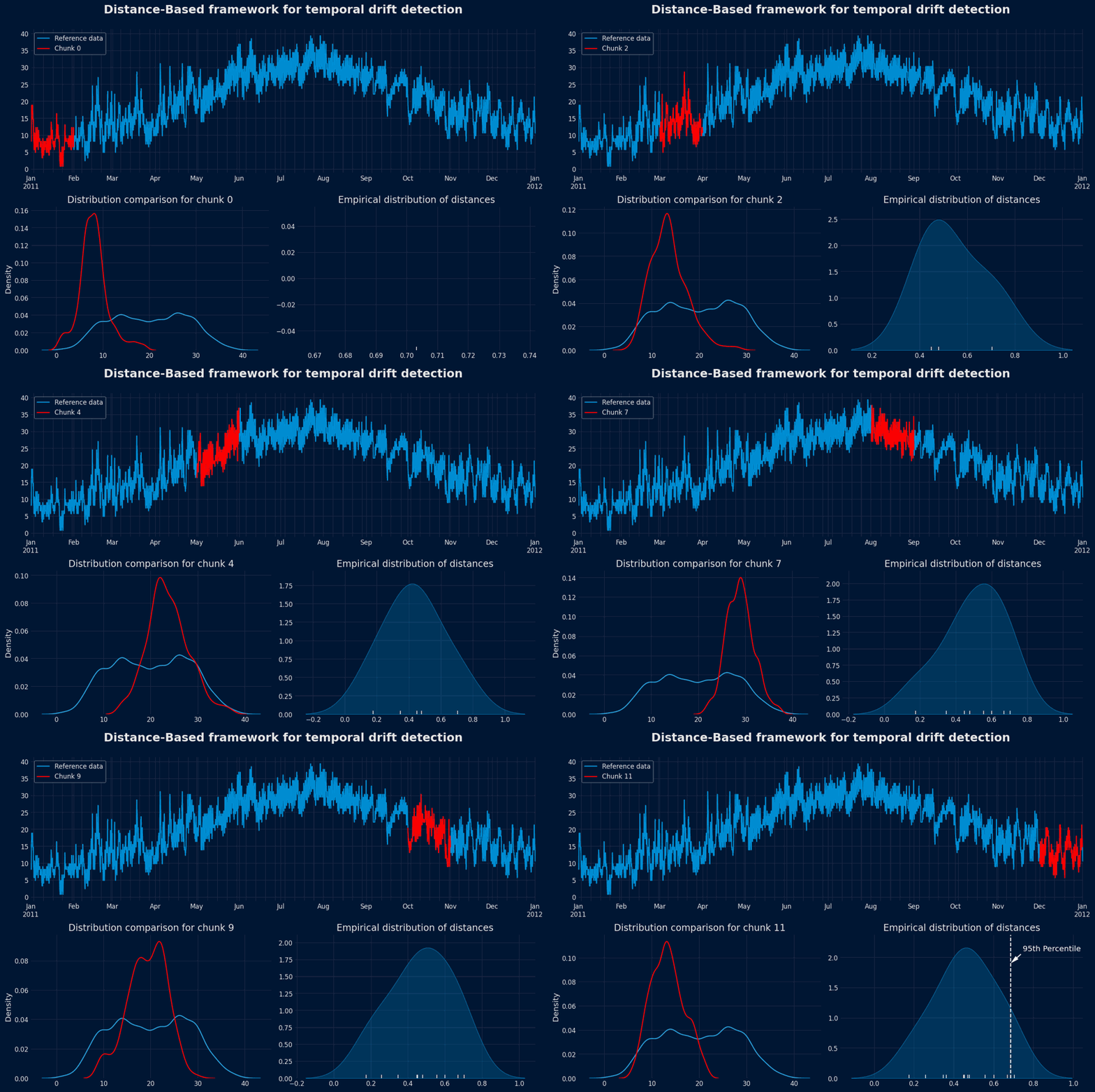
Population Drift Detection - Animation

2. Monitoring Phase: Detecting Drift in New Data¶

Once the baseline distribution is established, new data can be continuously evaluated for drift.

1. Chunk new data
   As new observations become available, segment them into chunks of the same length used in the reference phase: $$\{ C'_1, C'_2, \ldots, C'_m \}$$

2. Compute distances to the reference
   For each new chunk $C'_j$, compute its distance to the reference baseline (either to all reference chunks or to an aggregated representation of the reference distribution).

3. Compare against the threshold

   • If $d(C'_j, \text{reference}) \leq \tau$, the data is consistent with the reference distribution.
   • If $d(C'_j, \text{reference}) > \tau$, flag the chunk as exhibiting potential drift.

4. Interpretation
   A flagged chunk suggests that the new data segment differs significantly from historical norms, implying a possible covariate (feature) or label drift. Such cases may warrant further investigation, model retraining, or data pipeline adjustments.

Since this framework compares the distribution of each variable separately, it cannot detect concept drift: if the relationship between the predictors and the target changes while their distributions stay the same, no alarm is raised. To detect concept drift, monitor the forecasting error of the model over time (for example, the MAE of the most recent predictions compared with the error obtained during backtesting).