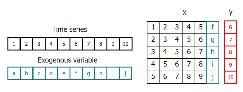
Exogenous variables (features)¶

Exogenous variables are predictors that are independent of the model being used for forecasting, and their future values must be known in order to include them in the prediction process. The inclusion of exogenous variables can enhance the accuracy of forecasts.

In Skforecast, exogenous variables can be easily included as predictors in all forecasting models. To ensure that their effects are accurately accounted for, it is crucial to include these variables during both the training and prediction phases. This will help to optimize the accuracy of forecasts and provide more reliable predictions.

  Note

When exogenous variables are used, their values must be aligned so that y[i] regresses on exog[i].

Time series transformation including an exogenous variable.

  Warning

When exogenous variables are included in a forecasting model, it is assumed that all exogenous inputs are known in the future. Do not include exogenous variables as predictors if their future value will not be known when making predictions.

Libraries¶

In [1]:

# Libraries
# ==============================================================================
import pandas as pd
import matplotlib.pyplot as plt
from skforecast.ForecasterAutoreg import ForecasterAutoreg
from sklearn.ensemble import RandomForestRegressor
from sklearn.metrics import mean_squared_error

# Libraries # ============================================================================== import pandas as pd import matplotlib.pyplot as plt from skforecast.ForecasterAutoreg import ForecasterAutoreg from sklearn.ensemble import RandomForestRegressor from sklearn.metrics import mean_squared_error

Data¶

In [2]:

# Download data
# ==============================================================================
url = (
    'https://raw.githubusercontent.com/JoaquinAmatRodrigo/skforecast/master/'
    'data/h2o_exog.csv'
)
data = pd.read_csv(
            url, sep=',', header=0, names=['datetime', 'y', 'exog_1', 'exog_2']
       )

# Data preprocessing
# ==============================================================================
data['datetime'] = pd.to_datetime(data['datetime'], format='%Y-%m-%d')
data = data.set_index('datetime')
data = data.asfreq('MS')
data = data.sort_index()

# Plot
# ==============================================================================
fig, ax=plt.subplots(figsize=(7, 3.5))
data.plot(ax=ax);

# Download data # ============================================================================== url = ( 'https://raw.githubusercontent.com/JoaquinAmatRodrigo/skforecast/master/' 'data/h2o_exog.csv' ) data = pd.read_csv( url, sep=',', header=0, names=['datetime', 'y', 'exog_1', 'exog_2'] ) # Data preprocessing # ============================================================================== data['datetime'] = pd.to_datetime(data['datetime'], format='%Y-%m-%d') data = data.set_index('datetime') data = data.asfreq('MS') data = data.sort_index() # Plot # ============================================================================== fig, ax=plt.subplots(figsize=(7, 3.5)) data.plot(ax=ax);

In [3]:

# Split data in train and test
# ==============================================================================
steps = 36
data_train = data.iloc[:-steps, :]
data_test  = data.iloc[-steps:, :]

# Split data in train and test # ============================================================================== steps = 36 data_train = data.iloc[:-steps, :] data_test = data.iloc[-steps:, :]

Train forecaster¶

In [4]:

# Create and fit forecaster
# ==============================================================================
forecaster = ForecasterAutoreg(
                 regressor = RandomForestRegressor(random_state=123),
                 lags      = 15
             )

forecaster.fit(
    y    = data_train['y'],
    exog = data_train[['exog_1', 'exog_2']]
)

forecaster

# Create and fit forecaster # ============================================================================== forecaster = ForecasterAutoreg( regressor = RandomForestRegressor(random_state=123), lags = 15 ) forecaster.fit( y = data_train['y'], exog = data_train[['exog_1', 'exog_2']] ) forecaster

Out[4]:

================= 
ForecasterAutoreg 
================= 
Regressor: RandomForestRegressor(random_state=123) 
Lags: [ 1  2  3  4  5  6  7  8  9 10 11 12 13 14 15] 
Transformer for y: None 
Transformer for exog: None 
Window size: 15 
Weight function included: False 
Exogenous included: True 
Type of exogenous variable: <class 'pandas.core.frame.DataFrame'> 
Exogenous variables names: ['exog_1', 'exog_2'] 
Training range: [Timestamp('1992-04-01 00:00:00'), Timestamp('2005-06-01 00:00:00')] 
Training index type: DatetimeIndex 
Training index frequency: MS 
Regressor parameters: {'bootstrap': True, 'ccp_alpha': 0.0, 'criterion': 'squared_error', 'max_depth': None, 'max_features': 1.0, 'max_leaf_nodes': None, 'max_samples': None, 'min_impurity_decrease': 0.0, 'min_samples_leaf': 1, 'min_samples_split': 2, 'min_weight_fraction_leaf': 0.0, 'n_estimators': 100, 'n_jobs': None, 'oob_score': False, 'random_state': 123, 'verbose': 0, 'warm_start': False} 
fit_kwargs: {} 
Creation date: 2023-05-29 13:10:36 
Last fit date: 2023-05-29 13:10:36 
Skforecast version: 0.8.1 
Python version: 3.10.11 
Forecaster id: None 

Prediction¶

If the Forecaster has been trained using exogenous variables, they should be provided during the prediction phase.

In [5]:

# Predict
# ==============================================================================
steps = 36
predictions = forecaster.predict(
                  steps = steps,
                  exog = data_test[['exog_1', 'exog_2']]
              )

predictions.head(3)

# Predict # ============================================================================== steps = 36 predictions = forecaster.predict( steps = steps, exog = data_test[['exog_1', 'exog_2']] ) predictions.head(3)

Out[5]:

2005-07-01    0.908832
2005-08-01    0.953925
2005-09-01    1.100887
Freq: MS, Name: pred, dtype: float64

In [6]:

# Plot predictions
# ==============================================================================
fig, ax=plt.subplots(figsize=(7, 3.5))
data_train['y'].plot(ax=ax, label='train')
data_test['y'].plot(ax=ax, label='test')
predictions.plot(ax=ax, label='predictions')
ax.legend();

# Plot predictions # ============================================================================== fig, ax=plt.subplots(figsize=(7, 3.5)) data_train['y'].plot(ax=ax, label='train') data_test['y'].plot(ax=ax, label='test') predictions.plot(ax=ax, label='predictions') ax.legend();

In [7]:

# Prediction error
# ==============================================================================
error_mse = mean_squared_error(
                y_true = data_test['y'],
                y_pred = predictions
            )

print(f"Test error (mse): {error_mse}")

# Prediction error # ============================================================================== error_mse = mean_squared_error( y_true = data_test['y'], y_pred = predictions ) print(f"Test error (mse): {error_mse}")

Test error (mse): 0.004022228812838391

Feature importances¶

If exogenous variables are included as predictors, they have a value of feature importances.

In [8]:

forecaster.get_feature_importances()

forecaster.get_feature_importances()

Out[8]:

	feature	importance
0	lag_1	0.013354
1	lag_2	0.061120
2	lag_3	0.009086
3	lag_4	0.002721
4	lag_5	0.002478
5	lag_6	0.003155
6	lag_7	0.002179
7	lag_8	0.008154
8	lag_9	0.010319
9	lag_10	0.020587
10	lag_11	0.007036
11	lag_12	0.773389
12	lag_13	0.004583
13	lag_14	0.018127
14	lag_15	0.008732
15	exog_1	0.010364
16	exog_2	0.044616

In [9]:

%%html
<style>
.jupyter-wrapper .jp-CodeCell .jp-Cell-inputWrapper .jp-InputPrompt {display: none;}
</style>

%%html