Backtesting¶

In time series forecasting, backtesting refers to the process of validating a predictive model using historical data. The technique involves moving backwards in time, step-by-step, to assess how well a model would have performed if it had been used to make predictions during that time period. Backtesting is a form of cross-validation that is applied to previous periods in the time series.

The purpose of backtesting is to evaluate the accuracy and effectiveness of a model and identify any potential issues or areas of improvement. By testing the model on historical data, one can assess how well it performs on data that it has not seen before. This is an important step in the modeling process, as it helps to ensure that the model is robust and reliable.

Backtesting can be done using a variety of techniques, such as simple train-test splits or more sophisticated methods like rolling windows or expanding windows. The choice of method depends on the specific needs of the analysis and the characteristics of the time series data.

Overall, backtesting is an essential step in the development of a time series forecasting model. By rigorously testing the model on historical data, one can improve its accuracy and ensure that it is effective at predicting future values of the time series.

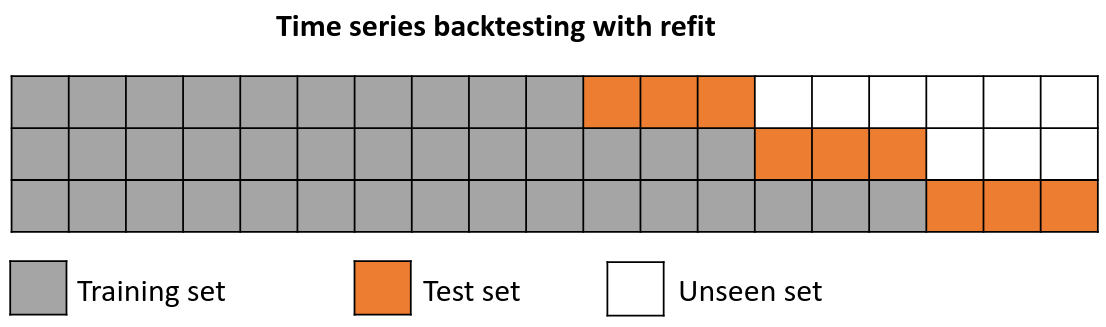
Backtesting with refit and increasing training size (fixed origin)¶

In this strategy, the model is trained before making predictions each time, and all available data up to that point is used in the training process. This differs from standard cross-validation, where the data is randomly distributed between training and validation sets.

Instead of randomizing the data, this backtesting sequentially increases the size of the training set while maintaining the temporal order of the data. By doing this, the model can be tested on progressively larger amounts of historical data, providing a more accurate assessment of its predictive capabilities.

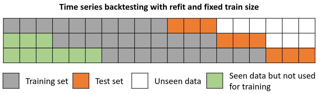
Backtesting with refit and increasing training size (fixed origin).

Backtesting with refit and fixed training size (rolling origin)¶

In this approach, the model is trained using a fixed window of past observations, and the testing is performed on a rolling basis, where the training window is moved forward in time. The size of the training window is kept constant, allowing for the model to be tested on different sections of the data. This technique is particularly useful when there is a limited amount of data available, or when the data is non-stationary, and the model's performance may vary over time. Is also known as time series cross-validation or walk-forward validation.

Backtesting with refit and fixed training size (rolling origin).

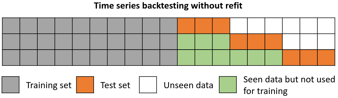
Backtesting without refit¶

Backtesting without refit is a strategy where the model is trained only once and used sequentially without updating it, following the temporal order of the data. This approach is advantageous as it is much faster than other methods that require retraining the model each time. However, the model may lose its predictive power over time as it does not incorporate the latest information available.

Backtesting without refit.

Backtesting including gap¶

This approach introduces a time gap between the training and test sets, replicating a scenario where predictions cannot be made immediately after the end of the training data.

For example, consider the goal of predicting the 24 hours of day D+1, but the predictions need to be made at 11:00 to allow sufficient flexibility. At 11:00 on day D, the task is to forecast hours [12 - 23] of the same day and hours [0 - 23] of day D+1. Thus, a total of 36 hours into the future must be predicted, with only the last 24 hours to be stored.

Backtesting with refit and gap.

Libraries¶

In [1]:

# Libraries
# ==============================================================================
import numpy as np
import pandas as pd
import matplotlib.pyplot as plt
from skforecast.ForecasterAutoreg import ForecasterAutoreg
from skforecast.model_selection import backtesting_forecaster
from sklearn.linear_model import Ridge
from sklearn.ensemble import RandomForestRegressor
from sklearn.metrics import mean_squared_error

# Libraries # ============================================================================== import numpy as np import pandas as pd import matplotlib.pyplot as plt from skforecast.ForecasterAutoreg import ForecasterAutoreg from skforecast.model_selection import backtesting_forecaster from sklearn.linear_model import Ridge from sklearn.ensemble import RandomForestRegressor from sklearn.metrics import mean_squared_error

Data¶

In [2]:

# Download data
# ==============================================================================
url = (
    'https://raw.githubusercontent.com/JoaquinAmatRodrigo/skforecast/master/'
    'data/h2o.csv'
)
data = pd.read_csv(url, sep=',', header=0, names=['y', 'datetime'])

# Data preprocessing
# ==============================================================================
data['datetime'] = pd.to_datetime(data['datetime'], format='%Y-%m-%d')
data = data.set_index('datetime')
data = data.asfreq('MS')
data = data[['y']]
data = data.sort_index()

# Train-validation dates
# ==============================================================================
end_train = '2002-01-01 23:59:00'

print(
    f"Train dates      : {data.index.min()} --- {data.loc[:end_train].index.max()}"
    f"  (n={len(data.loc[:end_train])})"
)
print(
    f"Validation dates : {data.loc[end_train:].index.min()} --- {data.index.max()}"
    f"  (n={len(data.loc[end_train:])})"
)

# Plot
# ==============================================================================
fig, ax = plt.subplots(figsize=(6, 3))
data.loc[:end_train].plot(ax=ax, label='train')
data.loc[end_train:].plot(ax=ax, label='validation')
ax.legend()
plt.show()

display(data.head(4))

# Download data # ============================================================================== url = ( 'https://raw.githubusercontent.com/JoaquinAmatRodrigo/skforecast/master/' 'data/h2o.csv' ) data = pd.read_csv(url, sep=',', header=0, names=['y', 'datetime']) # Data preprocessing # ============================================================================== data['datetime'] = pd.to_datetime(data['datetime'], format='%Y-%m-%d') data = data.set_index('datetime') data = data.asfreq('MS') data = data[['y']] data = data.sort_index() # Train-validation dates # ============================================================================== end_train = '2002-01-01 23:59:00' print( f"Train dates : {data.index.min()} --- {data.loc[:end_train].index.max()}" f" (n={len(data.loc[:end_train])})" ) print( f"Validation dates : {data.loc[end_train:].index.min()} --- {data.index.max()}" f" (n={len(data.loc[end_train:])})" ) # Plot # ============================================================================== fig, ax = plt.subplots(figsize=(6, 3)) data.loc[:end_train].plot(ax=ax, label='train') data.loc[end_train:].plot(ax=ax, label='validation') ax.legend() plt.show() display(data.head(4))

Train dates      : 1991-07-01 00:00:00 --- 2002-01-01 00:00:00  (n=127)
Validation dates : 2002-02-01 00:00:00 --- 2008-06-01 00:00:00  (n=77)

	y
datetime
1991-07-01	0.429795
1991-08-01	0.400906
1991-09-01	0.432159
1991-10-01	0.492543

Backtest¶

An example of a backtesting with refit consists of the following steps:

1. Train the model using an initial training set, the length of which is specified by initial_train_size.

2. Once the model is trained, it is used to make predictions for the next 10 steps (steps=10) in the data. These predictions are saved for later evaluation.

3. As refit is set to True, the size of the training set is increased by adding the lats 10 data points (the previously predicted 10 steps), while the next 10 steps are used as test data.

4. After expanding the training set, the model is retrained using the updated training data and then used to predict the next 10 steps.

5. Repeat steps 3 and 4 until the entire series has been tested.

By following these steps, you can ensure that the model is evaluated on multiple sets of test data, thereby providing a more accurate assessment of its predictive power.

In [3]:

# Backtesting forecaster
# ==============================================================================
forecaster = ForecasterAutoreg(
                 regressor = RandomForestRegressor(random_state=123),
                 lags      = 15 
             )

metric, predictions = backtesting_forecaster(
                          forecaster            = forecaster,
                          y                     = data['y'],
                          steps                 = 10,
                          metric                = 'mean_squared_error',
                          initial_train_size    = len(data.loc[:end_train]),
                          fixed_train_size      = False,
                          gap                   = 0,
                          allow_incomplete_fold = True,
                          refit                 = True,
                          verbose               = True,
                          show_progress         = True  
                      )

# Backtesting forecaster # ============================================================================== forecaster = ForecasterAutoreg( regressor = RandomForestRegressor(random_state=123), lags = 15 ) metric, predictions = backtesting_forecaster( forecaster = forecaster, y = data['y'], steps = 10, metric = 'mean_squared_error', initial_train_size = len(data.loc[:end_train]), fixed_train_size = False, gap = 0, allow_incomplete_fold = True, refit = True, verbose = True, show_progress = True )

Information of backtesting process
----------------------------------
Number of observations used for initial training: 127
Number of observations used for backtesting: 77
    Number of folds: 8
    Number of steps per fold: 10
    Number of steps to exclude from the end of each train set before test (gap): 0
    Last fold only includes 7 observations.

Fold: 0
    Training:   1991-07-01 00:00:00 -- 2002-01-01 00:00:00  (n=127)
    Validation: 2002-02-01 00:00:00 -- 2002-11-01 00:00:00  (n=10)
Fold: 1
    Training:   1991-07-01 00:00:00 -- 2002-11-01 00:00:00  (n=137)
    Validation: 2002-12-01 00:00:00 -- 2003-09-01 00:00:00  (n=10)
Fold: 2
    Training:   1991-07-01 00:00:00 -- 2003-09-01 00:00:00  (n=147)
    Validation: 2003-10-01 00:00:00 -- 2004-07-01 00:00:00  (n=10)
Fold: 3
    Training:   1991-07-01 00:00:00 -- 2004-07-01 00:00:00  (n=157)
    Validation: 2004-08-01 00:00:00 -- 2005-05-01 00:00:00  (n=10)
Fold: 4
    Training:   1991-07-01 00:00:00 -- 2005-05-01 00:00:00  (n=167)
    Validation: 2005-06-01 00:00:00 -- 2006-03-01 00:00:00  (n=10)
Fold: 5
    Training:   1991-07-01 00:00:00 -- 2006-03-01 00:00:00  (n=177)
    Validation: 2006-04-01 00:00:00 -- 2007-01-01 00:00:00  (n=10)
Fold: 6
    Training:   1991-07-01 00:00:00 -- 2007-01-01 00:00:00  (n=187)
    Validation: 2007-02-01 00:00:00 -- 2007-11-01 00:00:00  (n=10)
Fold: 7
    Training:   1991-07-01 00:00:00 -- 2007-11-01 00:00:00  (n=197)
    Validation: 2007-12-01 00:00:00 -- 2008-06-01 00:00:00  (n=7)

  0%|          | 0/8 [00:00<?, ?it/s]

In [4]:

print(f"Backtest error: {metric}")
predictions.head(4)

print(f"Backtest error: {metric}") predictions.head(4)

Backtest error: 0.00818535931502708

Out[4]:

	pred
2002-02-01	0.594506
2002-03-01	0.785886
2002-04-01	0.698925
2002-05-01	0.790560

In [5]:

# Plot predictions
# ==============================================================================
fig, ax = plt.subplots(figsize=(6, 3))
data.loc[end_train:, 'y'].plot(ax=ax)
predictions.plot(ax=ax)
ax.legend();

# Plot predictions # ============================================================================== fig, ax = plt.subplots(figsize=(6, 3)) data.loc[end_train:, 'y'].plot(ax=ax) predictions.plot(ax=ax) ax.legend();

Backtesting with gap¶

The gap size can be adjusted with the gap argument. In addition, the allow_incomplete_fold parameter allows the last fold to be excluded from the analysis if it doesn't have the same size as the required number of steps.

These arguments can be used in conjunction with either refit set to True or False, depending on the needs and objectives of the use case.

  Note

In this example, although only the last 10 predictions (steps) are stored for model evaluation, the total number of predicted steps in each fold is 15 (steps + gap).

In [6]:

# Backtesting forecaster
# ==============================================================================
forecaster = ForecasterAutoreg(
                 regressor = RandomForestRegressor(random_state=123),
                 lags      = 15 
             )

metric, predictions = backtesting_forecaster(
                          forecaster            = forecaster,
                          y                     = data['y'],
                          steps                 = 10,
                          metric                = 'mean_squared_error',
                          initial_train_size    = len(data.loc[:end_train]),
                          fixed_train_size      = False,
                          gap                   = 5,
                          allow_incomplete_fold = False,
                          refit                 = True,
                          verbose               = True,
                          show_progress         = False  
                      )

# Backtesting forecaster # ============================================================================== forecaster = ForecasterAutoreg( regressor = RandomForestRegressor(random_state=123), lags = 15 ) metric, predictions = backtesting_forecaster( forecaster = forecaster, y = data['y'], steps = 10, metric = 'mean_squared_error', initial_train_size = len(data.loc[:end_train]), fixed_train_size = False, gap = 5, allow_incomplete_fold = False, refit = True, verbose = True, show_progress = False )

Information of backtesting process
----------------------------------
Number of observations used for initial training: 127
Number of observations used for backtesting: 77
    Number of folds: 7
    Number of steps per fold: 10
    Number of steps to exclude from the end of each train set before test (gap): 5
    Last fold has been excluded because it was incomplete.

Fold: 0
    Training:   1991-07-01 00:00:00 -- 2002-01-01 00:00:00  (n=127)
    Validation: 2002-07-01 00:00:00 -- 2003-04-01 00:00:00  (n=10)
Fold: 1
    Training:   1991-07-01 00:00:00 -- 2002-11-01 00:00:00  (n=137)
    Validation: 2003-05-01 00:00:00 -- 2004-02-01 00:00:00  (n=10)
Fold: 2
    Training:   1991-07-01 00:00:00 -- 2003-09-01 00:00:00  (n=147)
    Validation: 2004-03-01 00:00:00 -- 2004-12-01 00:00:00  (n=10)
Fold: 3
    Training:   1991-07-01 00:00:00 -- 2004-07-01 00:00:00  (n=157)
    Validation: 2005-01-01 00:00:00 -- 2005-10-01 00:00:00  (n=10)
Fold: 4
    Training:   1991-07-01 00:00:00 -- 2005-05-01 00:00:00  (n=167)
    Validation: 2005-11-01 00:00:00 -- 2006-08-01 00:00:00  (n=10)
Fold: 5
    Training:   1991-07-01 00:00:00 -- 2006-03-01 00:00:00  (n=177)
    Validation: 2006-09-01 00:00:00 -- 2007-06-01 00:00:00  (n=10)
Fold: 6
    Training:   1991-07-01 00:00:00 -- 2007-01-01 00:00:00  (n=187)
    Validation: 2007-07-01 00:00:00 -- 2008-04-01 00:00:00  (n=10)

In [7]:

print(f"Backtest error: {metric}")
predictions.head(4)

print(f"Backtest error: {metric}") predictions.head(4)

Backtest error: 0.011194317866594718

Out[7]:

	pred
2002-07-01	0.870897
2002-08-01	0.920207
2002-09-01	0.942503
2002-10-01	1.022695

Backtesting with prediction intervals¶

Backtesting can be used not only to obtain point estimate predictions but also to obtain prediction intervals. Prediction intervals provide a range of values within which the actual values are expected to fall with a certain level of confidence. By estimating prediction intervals during backtesting, one can get a better understanding of the uncertainty associated with your model's predictions. This information can be used to assess the reliability of the model's predictions and to make more informed decisions. To learn more about probabilistic forecasting, visit Probabilistic forecasting.

In [8]:

# Backtesting forecaster with prediction intervals
# ==============================================================================
forecaster = ForecasterAutoreg(
                 regressor = Ridge(),
                 lags      = 15 
             )

metric, predictions = backtesting_forecaster(
                          forecaster            = forecaster,
                          y                     = data['y'],
                          steps                 = 10,
                          metric                = 'mean_squared_error',
                          initial_train_size    = len(data.loc[:end_train]),
                          fixed_train_size      = False,
                          gap                   = 0,
                          allow_incomplete_fold = True,
                          refit                 = True,
                          interval              = [5, 95],
                          n_boot                = 500,
                          verbose               = True,
                          show_progress         = False
                      )

# Backtesting forecaster with prediction intervals # ============================================================================== forecaster = ForecasterAutoreg( regressor = Ridge(), lags = 15 ) metric, predictions = backtesting_forecaster( forecaster = forecaster, y = data['y'], steps = 10, metric = 'mean_squared_error', initial_train_size = len(data.loc[:end_train]), fixed_train_size = False, gap = 0, allow_incomplete_fold = True, refit = True, interval = [5, 95], n_boot = 500, verbose = True, show_progress = False )

Information of backtesting process
----------------------------------
Number of observations used for initial training: 127
Number of observations used for backtesting: 77
    Number of folds: 8
    Number of steps per fold: 10
    Number of steps to exclude from the end of each train set before test (gap): 0
    Last fold only includes 7 observations.

Fold: 0
    Training:   1991-07-01 00:00:00 -- 2002-01-01 00:00:00  (n=127)
    Validation: 2002-02-01 00:00:00 -- 2002-11-01 00:00:00  (n=10)
Fold: 1
    Training:   1991-07-01 00:00:00 -- 2002-11-01 00:00:00  (n=137)
    Validation: 2002-12-01 00:00:00 -- 2003-09-01 00:00:00  (n=10)
Fold: 2
    Training:   1991-07-01 00:00:00 -- 2003-09-01 00:00:00  (n=147)
    Validation: 2003-10-01 00:00:00 -- 2004-07-01 00:00:00  (n=10)
Fold: 3
    Training:   1991-07-01 00:00:00 -- 2004-07-01 00:00:00  (n=157)
    Validation: 2004-08-01 00:00:00 -- 2005-05-01 00:00:00  (n=10)
Fold: 4
    Training:   1991-07-01 00:00:00 -- 2005-05-01 00:00:00  (n=167)
    Validation: 2005-06-01 00:00:00 -- 2006-03-01 00:00:00  (n=10)
Fold: 5
    Training:   1991-07-01 00:00:00 -- 2006-03-01 00:00:00  (n=177)
    Validation: 2006-04-01 00:00:00 -- 2007-01-01 00:00:00  (n=10)
Fold: 6
    Training:   1991-07-01 00:00:00 -- 2007-01-01 00:00:00  (n=187)
    Validation: 2007-02-01 00:00:00 -- 2007-11-01 00:00:00  (n=10)
Fold: 7
    Training:   1991-07-01 00:00:00 -- 2007-11-01 00:00:00  (n=197)
    Validation: 2007-12-01 00:00:00 -- 2008-06-01 00:00:00  (n=7)

In [9]:

predictions.head()

predictions.head()

Out[9]:

	pred	lower_bound	upper_bound
2002-02-01	0.703579	0.599636	0.834616
2002-03-01	0.673522	0.572605	0.787942
2002-04-01	0.698319	0.589196	0.815748
2002-05-01	0.703042	0.593719	0.831795
2002-06-01	0.733776	0.632476	0.842865

In [10]:

# Plot prediction intervals
# ==============================================================================
fig, ax = plt.subplots(figsize=(6, 3))
data.loc[end_train:, 'y'].plot(ax=ax, label='test')
predictions['pred'].plot(ax=ax, label='predictions')
ax.fill_between(
    predictions.index,
    predictions['lower_bound'],
    predictions['upper_bound'],
    color = 'red',
    alpha = 0.2,
    label = 'prediction interval'
)
ax.legend();

# Plot prediction intervals # ============================================================================== fig, ax = plt.subplots(figsize=(6, 3)) data.loc[end_train:, 'y'].plot(ax=ax, label='test') predictions['pred'].plot(ax=ax, label='predictions') ax.fill_between( predictions.index, predictions['lower_bound'], predictions['upper_bound'], color = 'red', alpha = 0.2, label = 'prediction interval' ) ax.legend();

Backtesting with exogenous variables¶

All the backtesting strategies discussed in this document can also be applied when incorporating exogenous variables in the forecasting model.

Exogenous variables are additional independent variables that can impact the value of the target variable being forecasted. These variables can provide valuable information to the model and improve its forecasting accuracy.

In [11]:

# Download data
# ==============================================================================
url = (
    'https://raw.githubusercontent.com/JoaquinAmatRodrigo/skforecast/master/'
    'data/h2o_exog.csv'
)
data = pd.read_csv(url, sep=',', header=0, names=['datetime', 'y', 'exog_1', 'exog_2'])

# Data preprocessing
# ==============================================================================
data['datetime'] = pd.to_datetime(data['datetime'], format='%Y-%m-%d')
data = data.set_index('datetime')
data = data.asfreq('MS')
data = data.sort_index()

# Train-validation dates
# ==============================================================================
end_train = '2002-01-01 23:59:00'

print(
    f"Train dates      : {data.index.min()} --- {data.loc[:end_train].index.max()}"
    f"  (n={len(data.loc[:end_train])})"
)
print(
    f"Validation dates : {data.loc[end_train:].index.min()} --- {data.index.max()}"
    f"  (n={len(data.loc[end_train:])})"
)

# Plot
# ==============================================================================
fig, ax=plt.subplots(figsize=(6, 3))
data.plot(ax=ax);

# Download data # ============================================================================== url = ( 'https://raw.githubusercontent.com/JoaquinAmatRodrigo/skforecast/master/' 'data/h2o_exog.csv' ) data = pd.read_csv(url, sep=',', header=0, names=['datetime', 'y', 'exog_1', 'exog_2']) # Data preprocessing # ============================================================================== data['datetime'] = pd.to_datetime(data['datetime'], format='%Y-%m-%d') data = data.set_index('datetime') data = data.asfreq('MS') data = data.sort_index() # Train-validation dates # ============================================================================== end_train = '2002-01-01 23:59:00' print( f"Train dates : {data.index.min()} --- {data.loc[:end_train].index.max()}" f" (n={len(data.loc[:end_train])})" ) print( f"Validation dates : {data.loc[end_train:].index.min()} --- {data.index.max()}" f" (n={len(data.loc[end_train:])})" ) # Plot # ============================================================================== fig, ax=plt.subplots(figsize=(6, 3)) data.plot(ax=ax);

Train dates      : 1992-04-01 00:00:00 --- 2002-01-01 00:00:00  (n=118)
Validation dates : 2002-02-01 00:00:00 --- 2008-06-01 00:00:00  (n=77)

In [12]:

# Backtest forecaster exogenous variables
# ==============================================================================
forecaster = ForecasterAutoreg(
                 regressor = RandomForestRegressor(random_state=123),
                 lags      = 15 
             )

metric, predictions = backtesting_forecaster(
                          forecaster            = forecaster,
                          y                     = data['y'],
                          exog                  = data[['exog_1', 'exog_2']],
                          steps                 = 10,
                          metric                = 'mean_squared_error',
                          initial_train_size    = len(data.loc[:end_train]),
                          fixed_train_size      = False,
                          gap                   = 0,
                          allow_incomplete_fold = True,
                          refit                 = True,
                          verbose               = True,
                          show_progress         = False
                      )

# Backtest forecaster exogenous variables # ============================================================================== forecaster = ForecasterAutoreg( regressor = RandomForestRegressor(random_state=123), lags = 15 ) metric, predictions = backtesting_forecaster( forecaster = forecaster, y = data['y'], exog = data[['exog_1', 'exog_2']], steps = 10, metric = 'mean_squared_error', initial_train_size = len(data.loc[:end_train]), fixed_train_size = False, gap = 0, allow_incomplete_fold = True, refit = True, verbose = True, show_progress = False )

Information of backtesting process
----------------------------------
Number of observations used for initial training: 118
Number of observations used for backtesting: 77
    Number of folds: 8
    Number of steps per fold: 10
    Number of steps to exclude from the end of each train set before test (gap): 0
    Last fold only includes 7 observations.

Fold: 0
    Training:   1992-04-01 00:00:00 -- 2002-01-01 00:00:00  (n=118)
    Validation: 2002-02-01 00:00:00 -- 2002-11-01 00:00:00  (n=10)
Fold: 1
    Training:   1992-04-01 00:00:00 -- 2002-11-01 00:00:00  (n=128)
    Validation: 2002-12-01 00:00:00 -- 2003-09-01 00:00:00  (n=10)
Fold: 2
    Training:   1992-04-01 00:00:00 -- 2003-09-01 00:00:00  (n=138)
    Validation: 2003-10-01 00:00:00 -- 2004-07-01 00:00:00  (n=10)
Fold: 3
    Training:   1992-04-01 00:00:00 -- 2004-07-01 00:00:00  (n=148)
    Validation: 2004-08-01 00:00:00 -- 2005-05-01 00:00:00  (n=10)
Fold: 4
    Training:   1992-04-01 00:00:00 -- 2005-05-01 00:00:00  (n=158)
    Validation: 2005-06-01 00:00:00 -- 2006-03-01 00:00:00  (n=10)
Fold: 5
    Training:   1992-04-01 00:00:00 -- 2006-03-01 00:00:00  (n=168)
    Validation: 2006-04-01 00:00:00 -- 2007-01-01 00:00:00  (n=10)
Fold: 6
    Training:   1992-04-01 00:00:00 -- 2007-01-01 00:00:00  (n=178)
    Validation: 2007-02-01 00:00:00 -- 2007-11-01 00:00:00  (n=10)
Fold: 7
    Training:   1992-04-01 00:00:00 -- 2007-11-01 00:00:00  (n=188)
    Validation: 2007-12-01 00:00:00 -- 2008-06-01 00:00:00  (n=7)

In [13]:

print(f"Backtest error with exogenous variables: {metric}")

print(f"Backtest error with exogenous variables: {metric}")

Backtest error with exogenous variables: 0.007800037462113706

In [14]:

fig, ax = plt.subplots(figsize=(6, 3))
data.loc[end_train:].plot(ax=ax)
predictions.plot(ax=ax)
ax.legend(loc="upper left");

fig, ax = plt.subplots(figsize=(6, 3)) data.loc[end_train:].plot(ax=ax) predictions.plot(ax=ax) ax.legend(loc="upper left");

Backtesting with custom metric¶

In addition to the commonly used metrics such as mean_squared_error, mean_absolute_error, and mean_absolute_percentage_error, users have the flexibility to define their own custom metric function, provided that it includes the arguments y_true (the true values of the series) and y_pred (the predicted values), and returns a numeric value (either a float or an int).

This customizability enables users to evaluate the model's predictive performance in a wide range of scenarios, such as considering only certain months, days, non holiday; or focusing only on the last step of the predicted horizon.

To illustrate this, consider the following example: a 12-month horizon is forecasted, but the interest metric is calculated by considering only the last three months of each year. This is achieved by defining a custom metric function that takes into account only the relevant months, which is then passed as an argument to the backtesting function.

In [15]:

# Backtesting with custom metric
# ==============================================================================
def custom_metric(y_true, y_pred):
    """
    Calculate the mean squared error using only the predicted values of the last
    3 months of the year.
    """
    mask = y_true.index.month.isin([10, 11, 12])
    metric = mean_squared_error(y_true[mask], y_pred[mask])
    
    return metric


metric, predictions = backtesting_forecaster(
                          forecaster            = forecaster,
                          y                     = data['y'],
                          steps                 = 10,
                          metric                = custom_metric,
                          initial_train_size    = len(data.loc[:end_train]),
                          fixed_train_size      = False,
                          gap                   = 0,
                          allow_incomplete_fold = True,
                          refit                 = True,
                          verbose               = False,
                          show_progress         = False
                      )

print(f"Backtest error custom metric: {metric}")

# Backtesting with custom metric # ============================================================================== def custom_metric(y_true, y_pred): """ Calculate the mean squared error using only the predicted values of the last 3 months of the year. """ mask = y_true.index.month.isin([10, 11, 12]) metric = mean_squared_error(y_true[mask], y_pred[mask]) return metric metric, predictions = backtesting_forecaster( forecaster = forecaster, y = data['y'], steps = 10, metric = custom_metric, initial_train_size = len(data.loc[:end_train]), fixed_train_size = False, gap = 0, allow_incomplete_fold = True, refit = True, verbose = False, show_progress = False ) print(f"Backtest error custom metric: {metric}")

Backtest error custom metric: 0.005482666107945366

Backtesting with multiple metrics¶

The backtesting_forecaster function provides a convenient way to estimate multiple metrics simultaneously by accepting a list of metrics as an input argument. This list can include any combination of built-in metrics, such as mean_squared_error, mean_absolute_error, and mean_absolute_percentage_error, as well as user-defined custom metrics.

By specifying multiple metrics, users can obtain a more comprehensive evaluation of the model's predictive performance, which can help in selecting the best model for a particular task. Additionally, the ability to include custom metrics allows users to tailor the evaluation to specific use cases and domain-specific requirements.

In [16]:

metrics, predictions = backtesting_forecaster(
                           forecaster            = forecaster,
                           y                     = data['y'],
                           steps                 = 10,
                           metric                = ['mean_squared_error', 'mean_absolute_error'],
                           initial_train_size    = len(data.loc[:end_train]),
                           fixed_train_size      = False,
                           gap                   = 0,
                           allow_incomplete_fold = True,
                           refit                 = True,
                           verbose               = False,
                           show_progress         = False
                       )

print(f"Backtest error metrics: {metrics}")

metrics, predictions = backtesting_forecaster( forecaster = forecaster, y = data['y'], steps = 10, metric = ['mean_squared_error', 'mean_absolute_error'], initial_train_size = len(data.loc[:end_train]), fixed_train_size = False, gap = 0, allow_incomplete_fold = True, refit = True, verbose = False, show_progress = False ) print(f"Backtest error metrics: {metrics}")

Backtest error metrics: [0.00804575658744146, 0.06502216041298702]

Backtesting on training data¶

While the main focus of creating forecasting models is predicting future values, it's also useful to evaluate whether the model is learning from the training data. Predictions on the training data can help with this evaluation.

To obtain predictions on the training data,the forecaster must first be fitted using the training dataset. Then, backtesting can be performed using backtesting_forecaster and specifying the arguments initial_train_size=None and refit=False. This configuration enables backtesting on the same data that was used to train the model.

In [17]:

# Create and fit forecaster
# ==============================================================================
forecaster = ForecasterAutoreg(
                 regressor = RandomForestRegressor(random_state=123),
                 lags      = 15 
             )

forecaster.fit(y=data['y'])

# Create and fit forecaster # ============================================================================== forecaster = ForecasterAutoreg( regressor = RandomForestRegressor(random_state=123), lags = 15 ) forecaster.fit(y=data['y'])

In [18]:

# Backtesting on training data
# ==============================================================================
metric, predictions_training = backtesting_forecaster(
                                   forecaster         = forecaster,
                                   y                  = data['y'],
                                   steps              = 1,
                                   metric             = 'mean_squared_error',
                                   initial_train_size = None,
                                   refit              = False,
                                   verbose            = False,
                                   show_progress      = False
                               )

print(f"Backtest training error: {metric}")

# Backtesting on training data # ============================================================================== metric, predictions_training = backtesting_forecaster( forecaster = forecaster, y = data['y'], steps = 1, metric = 'mean_squared_error', initial_train_size = None, refit = False, verbose = False, show_progress = False ) print(f"Backtest training error: {metric}")

Backtest training error: 0.0005647902993476632

In [19]:

predictions_training.head(4)

predictions_training.head(4)

Out[19]:

	pred
1993-07-01	0.515375
1993-08-01	0.558055
1993-09-01	0.597601
1993-10-01	0.618857

It is important to note that the first 15 observations are excluded from the predictions since they are required to generate the lags that serve as predictors in the model.

In [20]:

# Plot training predictions
# ==============================================================================
fig, ax = plt.subplots(figsize=(6, 3))
data['y'].plot(ax=ax)
predictions_training.plot(ax=ax)
ax.set_title("Backtesting on training data")
ax.legend();

# Plot training predictions # ============================================================================== fig, ax = plt.subplots(figsize=(6, 3)) data['y'].plot(ax=ax) predictions_training.plot(ax=ax) ax.set_title("Backtesting on training data") ax.legend();

In [21]:

%%html
<style>
.jupyter-wrapper .jp-CodeCell .jp-Cell-inputWrapper .jp-InputPrompt {display: none;}
</style>

%%html