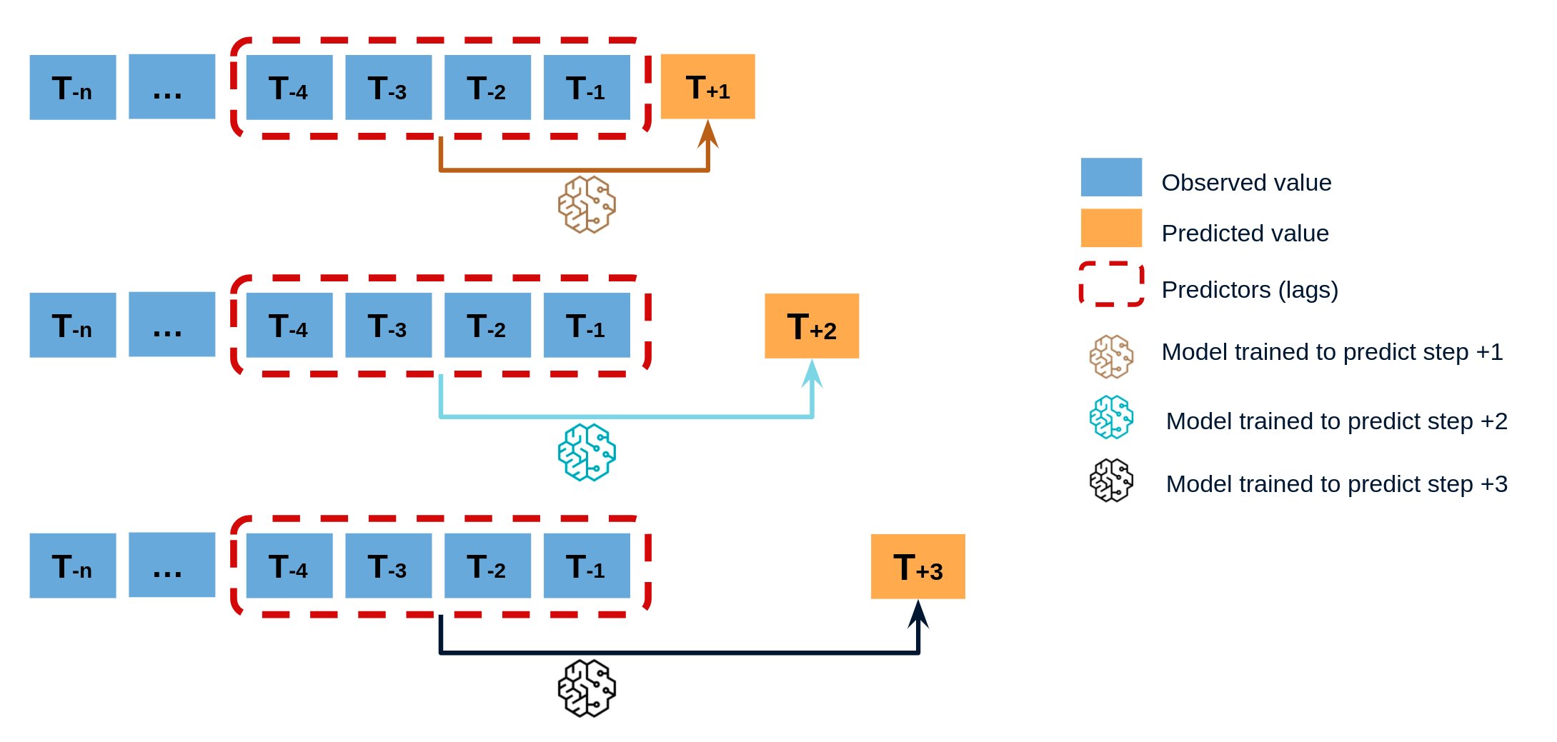
Direct multi-step forecaster¶

ForecasterAutoreg and ForecasterAutoregCustom models follow a recursive prediction strategy in which each new prediction builds on the previous one. An alternative is to train a model for each step that has to be predicted. This strategy, commonly known as direct multistep forecasting, is computationally more expensive than the recursive since it requires training several models. However, in some scenarios, it achieves better results. This type of model can be obtained with the ForecasterAutoregDirect class and can also include one or multiple exogenous variables.

To train a ForecasterAutoregDirect a different training matrix is created for each model.

Libraries¶

In [1]:

# Libraries
# ==============================================================================
import numpy as np
import pandas as pd
import matplotlib.pyplot as plt
from skforecast.ForecasterAutoregDirect import ForecasterAutoregDirect
from sklearn.linear_model import Ridge
from sklearn.metrics import mean_squared_error

# Libraries # ============================================================================== import numpy as np import pandas as pd import matplotlib.pyplot as plt from skforecast.ForecasterAutoregDirect import ForecasterAutoregDirect from sklearn.linear_model import Ridge from sklearn.metrics import mean_squared_error

Data¶

In [2]:

# Download data
# ==============================================================================
url = ('https://raw.githubusercontent.com/JoaquinAmatRodrigo/skforecast/master/data/h2o.csv')
data = pd.read_csv(url, sep=',', header=0, names=['y', 'datetime'])

# Data preprocessing
# ==============================================================================
data['datetime'] = pd.to_datetime(data['datetime'], format='%Y/%m/%d')
data = data.set_index('datetime')
data = data.asfreq('MS')
data = data['y']
data = data.sort_index()

# Split train-test
# ==============================================================================
steps = 36
data_train = data[:-steps]
data_test  = data[-steps:]

# Plot
# ==============================================================================
fig, ax=plt.subplots(figsize=(9, 4))
data_train.plot(ax=ax, label='train')
data_test.plot(ax=ax, label='test')
ax.legend();

# Download data # ============================================================================== url = ('https://raw.githubusercontent.com/JoaquinAmatRodrigo/skforecast/master/data/h2o.csv') data = pd.read_csv(url, sep=',', header=0, names=['y', 'datetime']) # Data preprocessing # ============================================================================== data['datetime'] = pd.to_datetime(data['datetime'], format='%Y/%m/%d') data = data.set_index('datetime') data = data.asfreq('MS') data = data['y'] data = data.sort_index() # Split train-test # ============================================================================== steps = 36 data_train = data[:-steps] data_test = data[-steps:] # Plot # ============================================================================== fig, ax=plt.subplots(figsize=(9, 4)) data_train.plot(ax=ax, label='train') data_test.plot(ax=ax, label='test') ax.legend();

Train forecaster¶

In [3]:

# Create and fit forecaster
# ==============================================================================
forecaster = ForecasterAutoregDirect(
                 regressor = Ridge(),
                 steps     = 36,
                 lags      = 15
             )

forecaster.fit(y=data_train)
forecaster

# Create and fit forecaster # ============================================================================== forecaster = ForecasterAutoregDirect( regressor = Ridge(), steps = 36, lags = 15 ) forecaster.fit(y=data_train) forecaster

Out[3]:

======================= 
ForecasterAutoregDirect 
======================= 
Regressor: Ridge() 
Lags: [ 1  2  3  4  5  6  7  8  9 10 11 12 13 14 15] 
Transformer for y: None 
Transformer for exog: None 
Window size: 15 
Maximum steps predicted: 36 
Included exogenous: False 
Type of exogenous variable: None 
Exogenous variables names: None 
Training range: [Timestamp('1991-07-01 00:00:00'), Timestamp('2005-06-01 00:00:00')] 
Training index type: DatetimeIndex 
Training index frequency: MS 
Regressor parameters: {'alpha': 1.0, 'copy_X': True, 'fit_intercept': True, 'max_iter': None, 'normalize': 'deprecated', 'positive': False, 'random_state': None, 'solver': 'auto', 'tol': 0.001} 
Creation date: 2022-09-24 08:27:36 
Last fit date: 2022-09-24 08:27:36 
Skforecast version: 0.5.0 
Python version: 3.9.13 

Prediction¶

In [4]:

# Predict
# ==============================================================================
steps = 36
predictions = forecaster.predict(steps=steps)
predictions.head(3)

# Predict # ============================================================================== steps = 36 predictions = forecaster.predict(steps=steps) predictions.head(3)

Out[4]:

2005-07-01    0.952051
2005-08-01    1.004145
2005-09-01    1.114590
Freq: MS, Name: pred, dtype: float64

In [5]:

# Plot predictions
# ==============================================================================
fig, ax=plt.subplots(figsize=(9, 4))
data_train.plot(ax=ax, label='train')
data_test.plot(ax=ax, label='test')
predictions.plot(ax=ax, label='predictions')
ax.legend();

# Plot predictions # ============================================================================== fig, ax=plt.subplots(figsize=(9, 4)) data_train.plot(ax=ax, label='train') data_test.plot(ax=ax, label='test') predictions.plot(ax=ax, label='predictions') ax.legend();

In [6]:

# Prediction error
# ==============================================================================
error_mse = mean_squared_error(
                y_true = data_test,
                y_pred = predictions
            )
print(f"Test error (mse): {error_mse}")

# Prediction error # ============================================================================== error_mse = mean_squared_error( y_true = data_test, y_pred = predictions ) print(f"Test error (mse): {error_mse}")

Test error (mse): 0.008419597278831958

Feature importance¶

Since ForecasterAutoregDirect fits one model per step, it is necessary to specify from which model retrieves its feature importance.

In [7]:

forecaster.get_feature_importance(step=1)

forecaster.get_feature_importance(step=1)

Out[7]:

	feature	importance
0	lag_1	0.139299
1	lag_2	0.051089
2	lag_3	0.044192
3	lag_4	-0.019868
4	lag_5	-0.017935
5	lag_6	-0.013233
6	lag_7	-0.021063
7	lag_8	-0.012591
8	lag_9	0.011918
9	lag_10	0.020511
10	lag_11	0.154030
11	lag_12	0.551652
12	lag_13	0.057513
13	lag_14	-0.071071
14	lag_15	-0.035237

Extract training matrix¶

Two steps are needed. One to create the whole training matrix and a second one to subset the data needed for each model (step).

In [8]:

X, y = forecaster.create_train_X_y(data_train)
# X and y to train model for step 1
X_1, y_1 = forecaster.filter_train_X_y_for_step(
               step    = 1,
               X_train = X,
               y_train = y,
           )

X_1.head(4)

X, y = forecaster.create_train_X_y(data_train) # X and y to train model for step 1 X_1, y_1 = forecaster.filter_train_X_y_for_step( step = 1, X_train = X, y_train = y, ) X_1.head(4)

Out[8]:

	lag_1	lag_2	lag_3	lag_4	lag_5	lag_6	lag_7	lag_8	lag_9	lag_10	lag_11	lag_12	lag_13	lag_14	lag_15
datetime
1995-09-01	0.534761	0.475463	0.483389	0.410534	0.361801	0.379808	0.351348	0.336220	0.660119	0.602652	0.502369	0.492543	0.432159	0.400906	0.429795
1995-10-01	0.568606	0.534761	0.475463	0.483389	0.410534	0.361801	0.379808	0.351348	0.336220	0.660119	0.602652	0.502369	0.492543	0.432159	0.400906
1995-11-01	0.595223	0.568606	0.534761	0.475463	0.483389	0.410534	0.361801	0.379808	0.351348	0.336220	0.660119	0.602652	0.502369	0.492543	0.432159
1995-12-01	0.771258	0.595223	0.568606	0.534761	0.475463	0.483389	0.410534	0.361801	0.379808	0.351348	0.336220	0.660119	0.602652	0.502369	0.492543

In [9]:

y_1.head(4)

y_1.head(4)

Out[9]:

datetime
1995-09-01    0.595223
1995-10-01    0.771258
1995-11-01    0.751503
1995-12-01    0.387554
Freq: MS, Name: y_step_1, dtype: float64

In [10]:

%%html
<style>
.jupyter-wrapper .jp-CodeCell .jp-Cell-inputWrapper .jp-InputPrompt {display: none;}
</style>

%%html