Time series aggregation¶

Time series aggregation involves summarizing or transforming data over specific time intervals. Two of the most common use cases are

• Aggregating data from one frequency to another. For example, converting hourly data to daily data.

• Aggregating data across a sliding window. For example, calculating a rolling average over the last 7 days.

These aggregations not only greatly reduce the total volume of data, but also help you find interesting features for your model faster.

Pandas provides an easy and efficient way to aggregate data from time series. This document shows how to use the resampling and rolling methods to aggregate data, with special emphasis on how to avoid data leakage, which is a common mistake when aggregating time series.

Libraries¶

In [1]:

# Libraries
# ==============================================================================
import pandas as pd
from skforecast.datasets import fetch_dataset

# Libraries # ============================================================================== import pandas as pd from skforecast.datasets import fetch_dataset

Data¶

In [2]:

# Download data
# ==============================================================================
data = fetch_dataset(name='vic_electricity')
data = data[['Demand', 'Temperature', 'Holiday']]
data.head(5)

# Download data # ============================================================================== data = fetch_dataset(name='vic_electricity') data = data[['Demand', 'Temperature', 'Holiday']] data.head(5)

vic_electricity
---------------
Half-hourly electricity demand for Victoria, Australia
O'Hara-Wild M, Hyndman R, Wang E, Godahewa R (2022).tsibbledata: Diverse
Datasets for 'tsibble'. https://tsibbledata.tidyverts.org/,
https://github.com/tidyverts/tsibbledata/.
https://tsibbledata.tidyverts.org/reference/vic_elec.html
Shape of the dataset: (52608, 4)

Out[2]:

	Demand	Temperature	Holiday
Time
2011-12-31 13:00:00	4382.825174	21.40	True
2011-12-31 13:30:00	4263.365526	21.05	True
2011-12-31 14:00:00	4048.966046	20.70	True
2011-12-31 14:30:00	3877.563330	20.55	True
2011-12-31 15:00:00	4036.229746	20.40	True

This dataset contains the electricity demand in Victoria (Australia) at half-hourly frequency.

In [3]:

# Index Frequency
# ==============================================================================
print(f"Frequency: {data.index.freq}")

# Index Frequency # ============================================================================== print(f"Frequency: {data.index.freq}")

Frequency: <30 * Minutes>

Change frequency (resample)¶

To change the frequency of a time series, use the resample method. This method allows you to specify a frequency and an aggregation function. It works similarly to the groupby method, but it works with time series indices.

When aggregating data, it is very important to use the closed and label arguments correctly. This avoids introducing future information into the training (data leakage).

• The closed argument specifies whether the interval is closed on the left-side, right-side, both or neither.

• The label argument specifies whether the result is labeled with the beginning or the end of the interval.

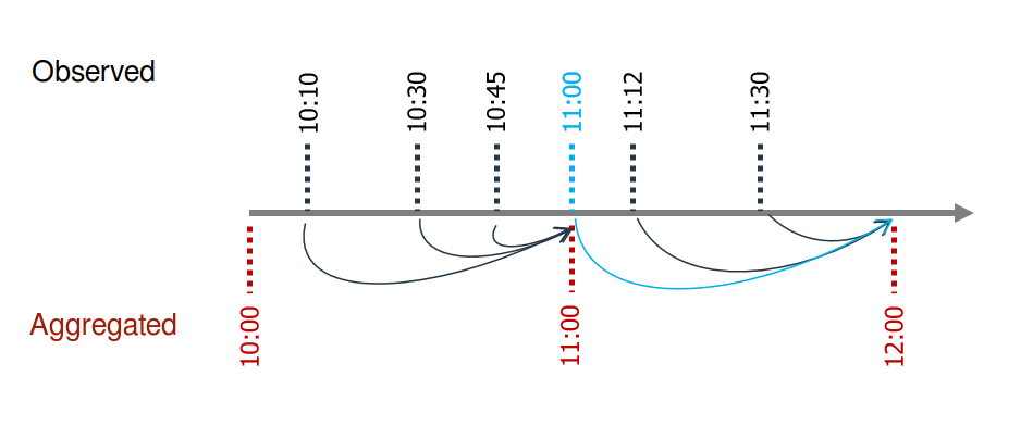
Suppose that values are available for 10:10, 10:30, 10:45, 11:00, 11:12, and 11:30. To obtain the hourly average, the value assigned to 11:00 must be calculated using the values for 10:10, 10:30, and 10:45; and the value assigned to 12:00 must be calculated using the value for 11:00, 11:12 and 11:30. The 11:00 average does not include the 11:00 point value because in reality the value is not available at that exact time.

In this case, the correct arguments are closed='left' and label='right'.

Diagram of data aggregation using the resample method without including future information.

For example, the code in the next cell converts the data from half-hourly to hourly frequency. Since there are multiple columns, an aggregation function must be specified for each column. In this case, the sum is calculated for the Demand column and the average is calculated for the rest.

In [4]:

# Aggregate data from 30 minutes to 1 hour
# ==============================================================================
data = data.resample(rule='1H', closed='left', label ='right').agg({
           'Demand': 'sum',
           'Temperature': 'mean',
           'Holiday': 'mean'
       })

data

# Aggregate data from 30 minutes to 1 hour # ============================================================================== data = data.resample(rule='1H', closed='left', label ='right').agg({ 'Demand': 'sum', 'Temperature': 'mean', 'Holiday': 'mean' }) data

C:\Users\jaesc2\AppData\Local\Temp\ipykernel_19428\1816291895.py:3: FutureWarning: 'H' is deprecated and will be removed in a future version, please use 'h' instead.
  data = data.resample(rule='1H', closed='left', label ='right').agg({

Out[4]:

	Demand	Temperature	Holiday
Time
2011-12-31 14:00:00	8646.190700	21.225	1.0
2011-12-31 15:00:00	7926.529376	20.625	1.0
2011-12-31 16:00:00	7901.826990	20.325	1.0
2011-12-31 17:00:00	7255.721350	19.850	1.0
2011-12-31 18:00:00	6792.503352	19.025	1.0
...	...	...	...
2014-12-31 09:00:00	8139.251100	21.600	0.0
2014-12-31 10:00:00	7818.461408	20.300	0.0
2014-12-31 11:00:00	7801.201802	19.650	0.0
2014-12-31 12:00:00	7516.472988	18.100	0.0
2014-12-31 13:00:00	7571.301440	17.200	0.0

26304 rows × 3 columns

Rolling window aggregation¶

Rolling window aggregation is used to calculate statistics over a sliding window of time. For example, the 24h rolling average is the average of the last 24 hours of data. As with the resample method, it is very important to use the closed='left' and center=False arguments correctly to avoid introducing future information into the training (data leakage).

In [5]:

# Rolling mean for 4 hours
# ==============================================================================
data.rolling(window=4, min_periods=4, closed='left', center=False).mean()

# Rolling mean for 4 hours # ============================================================================== data.rolling(window=4, min_periods=4, closed='left', center=False).mean()

Out[5]:

	Demand	Temperature	Holiday
Time
2011-12-31 14:00:00	NaN	NaN	NaN
2011-12-31 15:00:00	NaN	NaN	NaN
2011-12-31 16:00:00	NaN	NaN	NaN
2011-12-31 17:00:00	NaN	NaN	NaN
2011-12-31 18:00:00	7932.567104	20.50625	1.0
...	...	...	...
2014-12-31 09:00:00	8490.517461	23.71250	0.0
2014-12-31 10:00:00	8482.825404	23.41250	0.0
2014-12-31 11:00:00	8314.896216	22.67500	0.0
2014-12-31 12:00:00	8076.417548	21.30000	0.0
2014-12-31 13:00:00	7818.846825	19.91250	0.0

26304 rows × 3 columns

The average values for 2011-12-31 18:00:00 are calculated from the values of the previous 4 hours (from 14:00:00 to 17:00:00).

In [6]:

# '2011-12-31 18:00:00' mean
# ==============================================================================
data.iloc[0:4, :].mean()

# '2011-12-31 18:00:00' mean # ============================================================================== data.iloc[0:4, :].mean()

Out[6]:

Demand         7932.567104
Temperature      20.506250
Holiday           1.000000
dtype: float64

⚠ Warning

When transforming time series data, such as aggregating, it is very important to avoid data leakage, which means using information from the future to calculate the current value.