Forecasting with Deep Learning
Deep learning models have become increasingly popular for time series forecasting, especially when traditional statistical approaches struggle to capture non-linear relationships or complex temporal patterns. By leveraging neural network architectures, deep learning methods can automatically learn features and dependencies directly from raw data, offering significant advantages for large datasets, multivariate time series, and problems where classic models fall short.
Introduction to Recurrent Neural Networks (RNN), LSTM, and GRU
Recurrent Neural Networks (RNN) are a family of models specifically designed to work with sequential data, such as time series. Unlike traditional feedforward neural networks, which treat each input independently, RNNs introduce an internal memory that allows them to capture dependencies between elements of a sequence. This enables the model to leverage information from previous steps to improve future predictions.
The fundamental building block of an RNN is the recurrent cell, which receives two inputs at each time step: the current data point and the previous hidden state (the "memory" of the network). At every step, the hidden state is updated, storing relevant information about the sequence up to that point. This architecture allows RNNs to “remember” trends and patterns over time.
However, simple RNNs face difficulties when learning long-term dependencies due to issues like the vanishing or exploding gradient problem. To address these limitations, more advanced architectures such as Long Short-Term Memory (LSTM) and Gated Recurrent Unit (GRU) were developed. These variants are better at capturing complex and long-range patterns in time series data.
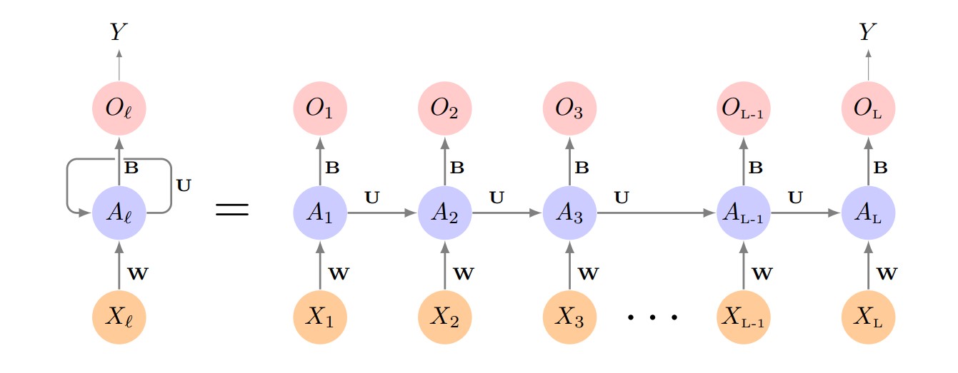
Basic RNN diagram. Source: James, G., Witten, D., Hastie, T., & Tibshirani, R. (2013). An introduction to statistical learning (1st ed.) [PDF]. Springer.
Types of Recurrent Layers in skforecast
With skforecast, you can use three main types of recurrent cells:
Simple RNN: Suitable for problems with short-term dependencies or when a simple model is sufficient. Less effective for capturing long-range patterns.
LSTM (Long Short-Term Memory): Adds gating mechanisms that allow the network to learn and retain information over longer periods. LSTMs are a popular choice for many complex forecasting problems.
GRU (Gated Recurrent Unit): Offers a simpler structure than LSTM, using fewer parameters while achieving comparable performance in many scenarios. Useful when computational efficiency is important.
✎ Note
Guidelines for choosing a recurrent layer:
- Use LSTM if your time series contains long-term patterns or complex dependencies.
- Try GRU as a lighter alternative to LSTM.
- Use Simple RNN only for straightforward tasks or as a baseline.
LSTM Architecture and Gates
Long Short-Term Memory (LSTM) networks are a widely used type of recurrent neural network designed to effectively capture long-range dependencies in sequential data. Unlike simple RNNs, LSTMs use a more sophisticated architecture based on a system of memory cells and gates that control the flow of information over time.
The core component of an LSTM is the memory cell, which maintains information across time steps. Three gates regulate how information is added, retained, or discarded at each step:
Forget Gate: Decides which information from the previous cell state should be removed. It uses the current input and previous hidden state, applying a sigmoid activation to produce a value between 0 and 1 (where 0 means “completely forget” and 1 means “completely keep”).
Input Gate: Controls how much new information is added to the cell state, again using the current input and previous hidden state with a sigmoid activation.
Output Gate: Determines how much of the cell state is exposed as output and passed to the next hidden state.
This gating mechanism enables LSTMs to selectively remember or forget information, making them highly effective for modeling sequences with long-term patterns.
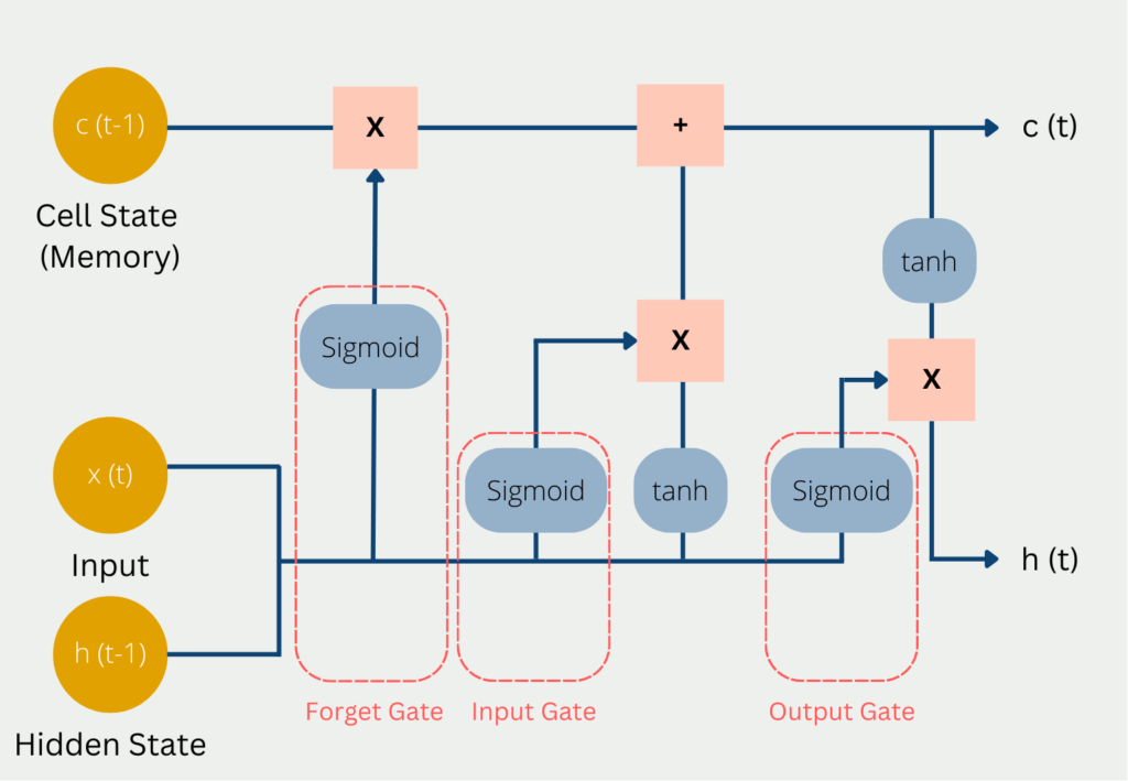
Diagram of the inputs and outputs of an LSTM. Source: codificandobits https://databasecamp.de/wp-content/uploads/lstm-architecture-1024x709.png.
Gated Recurrent Unit (GRU) cells are a simplified alternative to LSTMs, using only two gates (reset and update) but often achieving similar performance. GRUs require fewer parameters and can be computationally more efficient, which may be an advantage for some tasks or larger datasets.
💡 Tip
To learn more about forecasting with deep learning models visit our examples:
Libraries and data
⚠ Warning
skforecast supports multiple Keras backends: TensorFlow, JAX, and PyTorch (torch).
You can select the backend using the KERAS_BACKEND environment variable, or by editing your local configuration file at ~/.keras/keras.json.
import os
os.environ["KERAS_BACKEND"] = "tensorflow"  # Options: "tensorflow", "jax", or "torch"
import keras
The backend must be set before importing Keras in your Python session. Once Keras is imported, the backend cannot be changed without restarting your Python process.
Alternatively, you can set the backend in your configuration file at ~/.keras/keras.json:
{
    "backend": "tensorflow"  # Options: "tensorflow", "jax", or "torch"
}
# Libraries
# ==============================================================================
import os
os.environ["KERAS_BACKEND"] = "tensorflow"  # 'tensorflow', 'jax´ or 'torch'
import keras

import pandas as pd
import matplotlib.pyplot as plt
from sklearn.preprocessing import MinMaxScaler
from sklearn.pipeline import make_pipeline
from feature_engine.datetime import DatetimeFeatures
from feature_engine.creation import CyclicalFeatures

import skforecast
from skforecast.plot import set_dark_theme
from skforecast.datasets import fetch_dataset
from skforecast.deep_learning import create_and_compile_model
from skforecast.deep_learning import ForecasterRnn
from skforecast.model_selection import TimeSeriesFold
from skforecast.model_selection import backtesting_forecaster_multiseries
from skforecast.plot import plot_prediction_intervals

from keras.optimizers import Adam
from keras.losses import MeanSquaredError
from keras.callbacks import EarlyStopping, ReduceLROnPlateau

import warnings
warnings.filterwarnings('ignore', category=DeprecationWarning)

print(f"skforecast version: {skforecast.__version__}")
print(f"keras version: {keras.__version__}")
print(f"Using backend: {keras.backend.backend()}")
if keras.backend.backend() == "tensorflow":
    import tensorflow as tf
    print(f"tensorflow version: {tf.__version__}")
elif keras.backend.backend() == "torch":
    import torch
    print(f"torch version: {torch.__version__}")
else:
    print("Backend not recognized. Please use 'tensorflow' or 'torch'.")
skforecast version: 0.17.0
keras version: 3.10.0
Using backend: tensorflow
tensorflow version: 2.19.0
# Data download
# ==============================================================================
data = fetch_dataset(name="air_quality_valencia_no_missing")
data.head()
air_quality_valencia_no_missing
-------------------------------
Hourly measures of several air chemical pollutant at Valencia city (Avd.
Francia) from 2019-01-01 to 20213-12-31. Including the following variables:
pm2.5 (µg/m³), CO (mg/m³), NO (µg/m³), NO2 (µg/m³), PM10 (µg/m³), NOx (µg/m³),
O3 (µg/m³), Veloc. (m/s), Direc. (degrees), SO2 (µg/m³). Missing values have
been imputed using linear interpolation.
Red de Vigilancia y Control de la Contaminación Atmosférica, 46250047-València -
Av. França, https://mediambient.gva.es/es/web/calidad-ambiental/datos-
historicos.
Shape of the dataset: (43824, 10)
| so2 | co | no | no2 | pm10 | nox | o3 | veloc. | direc. | pm2.5 | |
|---|---|---|---|---|---|---|---|---|---|---|
| datetime | ||||||||||
| 2019-01-01 00:00:00 | 8.0 | 0.2 | 3.0 | 36.0 | 22.0 | 40.0 | 16.0 | 0.5 | 262.0 | 19.0 |
| 2019-01-01 01:00:00 | 8.0 | 0.1 | 2.0 | 40.0 | 32.0 | 44.0 | 6.0 | 0.6 | 248.0 | 26.0 |
| 2019-01-01 02:00:00 | 8.0 | 0.1 | 11.0 | 42.0 | 36.0 | 58.0 | 3.0 | 0.3 | 224.0 | 31.0 |
| 2019-01-01 03:00:00 | 10.0 | 0.1 | 15.0 | 41.0 | 35.0 | 63.0 | 3.0 | 0.2 | 220.0 | 30.0 |
| 2019-01-01 04:00:00 | 11.0 | 0.1 | 16.0 | 39.0 | 36.0 | 63.0 | 3.0 | 0.4 | 221.0 | 30.0 |
# Checking the frequency of the time series
# ==============================================================================
print(f"Index     : {data.index.dtype}")
print(f"Frequency : {data.index.freqstr}")
Index     : datetime64[ns]
Frequency : h
# Split train-validation-test
# ==============================================================================
data = data.loc["2019-01-01 00:00:00":"2021-12-31 23:59:59", :].copy()

end_train = "2021-03-31 23:59:00"
end_validation = "2021-09-30 23:59:00"
data_train = data.loc[:end_train, :].copy()
data_val = data.loc[end_train:end_validation, :].copy()
data_test = data.loc[end_validation:, :].copy()

print(
    f"Dates train      : {data_train.index.min()} --- "
    f"{data_train.index.max()}  (n={len(data_train)})"
)
print(
    f"Dates validation : {data_val.index.min()} --- "
    f"{data_val.index.max()}  (n={len(data_val)})"
)
print(
    f"Dates test       : {data_test.index.min()} --- "
    f"{data_test.index.max()}  (n={len(data_test)})"
)
Dates train      : 2019-01-01 00:00:00 --- 2021-03-31 23:00:00  (n=19704)
Dates validation : 2021-04-01 00:00:00 --- 2021-09-30 23:00:00  (n=4392)
Dates test       : 2021-10-01 00:00:00 --- 2021-12-31 23:00:00  (n=2208)
# Plot series
# ==============================================================================
set_dark_theme()
colors = plt.rcParams['axes.prop_cycle'].by_key()['color'] * 2
fig, axes = plt.subplots(len(data.columns), 1, figsize=(8, 8), sharex=True)

for i, col in enumerate(data.columns):
    axes[i].plot(data[col], label=col, color=colors[i])
    axes[i].legend(loc='upper right', fontsize=8)
    axes[i].tick_params(axis='both', labelsize=8)
    axes[i].axvline(pd.to_datetime(end_train), color='white', linestyle='--', linewidth=1)  # End train
    axes[i].axvline(pd.to_datetime(end_validation), color='white', linestyle='--', linewidth=1)  # End validation

fig.suptitle("Air Quality Valencia", fontsize=16)
plt.tight_layout()

Building RNN-based models easily with create_and_compile_model
skforecast provides the utility function create_and_compile_model to simplify the creation of recurrent neural network architectures (RNN, LSTM, or GRU) for time series forecasting. This function is designed to make it easy for both beginners and advanced users to build and compile Keras models with just a few lines of code.
Basic usage
For most forecasting scenarios, you can simply specify the time series data, the number of lagged observations, the number of steps to predict, and the type of recurrent layer you wish to use (LSTM, GRU, or SimpleRNN). By default, the function sets reasonable parameters for each layer, but all architectural details can be adjusted to fit specific requirements.
# Basic usage of `create_and_compile_model`
# ==============================================================================
model = create_and_compile_model(
            series          = data,    # All 10 series are used as predictors
            levels          = ["o3"],  # Target series to predict
            lags            = 32,      # Number of lags to use as predictors
            steps           = 24,      # Number of steps to predict
            recurrent_layer = "LSTM",  # Type of recurrent layer ('LSTM', 'GRU', or 'RNN')
            recurrent_units = 100,     # Number of units in the recurrent layer
            dense_units     = 64       # Number of units in the dense layer
        )

model.summary()
keras version: 3.10.0
Using backend: tensorflow
tensorflow version: 2.19.0
Model: "functional"
┏━━━━━━━━━━━━━━━━━━━━━━━━━━━━━━━━━┳━━━━━━━━━━━━━━━━━━━━━━━━┳━━━━━━━━━━━━━━━┓
┃ Layer (type)                    ┃ Output Shape           ┃       Param # ┃
┡━━━━━━━━━━━━━━━━━━━━━━━━━━━━━━━━━╇━━━━━━━━━━━━━━━━━━━━━━━━╇━━━━━━━━━━━━━━━┩
│ series_input (InputLayer)       │ (None, 32, 10)         │             0 │
├─────────────────────────────────┼────────────────────────┼───────────────┤
│ lstm_1 (LSTM)                   │ (None, 100)            │        44,400 │
├─────────────────────────────────┼────────────────────────┼───────────────┤
│ dense_1 (Dense)                 │ (None, 64)             │         6,464 │
├─────────────────────────────────┼────────────────────────┼───────────────┤
│ output_dense_td_layer (Dense)   │ (None, 24)             │         1,560 │
├─────────────────────────────────┼────────────────────────┼───────────────┤
│ reshape (Reshape)               │ (None, 24, 1)          │             0 │
└─────────────────────────────────┴────────────────────────┴───────────────┘
Total params: 52,424 (204.78 KB)
Trainable params: 52,424 (204.78 KB)
Non-trainable params: 0 (0.00 B)
Advanced customization
All arguments controlling layer types, units, activations, and other options can be customized. You may also pass your own Keras model if you need full flexibility beyond what the helper function provides.
The arguments recurrent_layers_kwargs and dense_layers_kwargs allow you to specify the parameters for the recurrent and dense layers, respectively.
When using a dictionary, the kwargs are replayed for each layer of the same type. For example, if you specify
recurrent_layers_kwargs = {'activation': 'tanh'}, all recurrent layers will use thetanhactivation function.You can also pass a list of dictionaries to specify different parameters for each layer. For instance,
recurrent_layers_kwargs = [{'activation': 'tanh'}, {'activation': 'relu'}]will specify that the first recurrent layer uses thetanhactivation function and the second usesrelu.
# Advance usage of `create_and_compile_model`
# ==============================================================================
model = create_and_compile_model(
    series                    = data,
    levels                    = ["o3"],
    lags                      = 32,
    steps                     = 24,
    exog                      = None,  # No exogenous variables
    recurrent_layer           = "LSTM",
    recurrent_units           = [128, 64],
    recurrent_layers_kwargs   = [{'activation': 'tanh'}, {'activation': 'relu'}],
    dense_units               = [128, 64],
    dense_layers_kwargs       = {'activation': 'relu'},
    output_dense_layer_kwargs = {'activation': 'linear'},
    compile_kwargs            = {'optimizer': Adam(learning_rate=0.001), 'loss': MeanSquaredError()},
    model_name                = None
)

model.summary()
keras version: 3.10.0
Using backend: tensorflow
tensorflow version: 2.19.0
Model: "functional_1"
┏━━━━━━━━━━━━━━━━━━━━━━━━━━━━━━━━━┳━━━━━━━━━━━━━━━━━━━━━━━━┳━━━━━━━━━━━━━━━┓
┃ Layer (type)                    ┃ Output Shape           ┃       Param # ┃
┡━━━━━━━━━━━━━━━━━━━━━━━━━━━━━━━━━╇━━━━━━━━━━━━━━━━━━━━━━━━╇━━━━━━━━━━━━━━━┩
│ series_input (InputLayer)       │ (None, 32, 10)         │             0 │
├─────────────────────────────────┼────────────────────────┼───────────────┤
│ lstm_1 (LSTM)                   │ (None, 32, 128)        │        71,168 │
├─────────────────────────────────┼────────────────────────┼───────────────┤
│ lstm_2 (LSTM)                   │ (None, 64)             │        49,408 │
├─────────────────────────────────┼────────────────────────┼───────────────┤
│ dense_1 (Dense)                 │ (None, 128)            │         8,320 │
├─────────────────────────────────┼────────────────────────┼───────────────┤
│ dense_2 (Dense)                 │ (None, 64)             │         8,256 │
├─────────────────────────────────┼────────────────────────┼───────────────┤
│ output_dense_td_layer (Dense)   │ (None, 24)             │         1,560 │
├─────────────────────────────────┼────────────────────────┼───────────────┤
│ reshape (Reshape)               │ (None, 24, 1)          │             0 │
└─────────────────────────────────┴────────────────────────┴───────────────┘
Total params: 138,712 (541.84 KB)
Trainable params: 138,712 (541.84 KB)
Non-trainable params: 0 (0.00 B)
To gain a deeper understanding of this function, refer to a later section of this guide: Understanding create_and_compile_model in depth.
If you need to define a completely custom architecture, you can create your own Keras model and use it directly in skforecast workflows.
# Plotting the model architecture (require `pydot` and `graphviz`)
# ==============================================================================
# from keras.utils import plot_model
# plot_model(model, show_shapes=True, show_layer_names=True, to_file='model-architecture.png')
Types of problems in time series forecasting
Deep learning models for time series can handle a wide variety of forecasting scenarios, depending on how you structure your input data and define your prediction targets. These models are flexible enough to:
Predict a single value or multiple future values (single-step vs multi-step forecasting).
Work with a single time series or multiple series (both as predictors and as targets).
Incorporate exogenous variables (external features or known future information) alongside your main time series data.
By adjusting your data inputs (number of series, steps ahead to predict, and exogenous variables) deep learning architectures can be adapted to solve almost any classical or advanced forecasting problem.
1. Single-Series, Single-Step Forecasting (1:1)
In this scenario, the goal is to predict the next value in a single time series, using only its own past observations as predictors. This is known as a univariate autoregressive forecasting problem.
For example: Given a sequence of values ${y_{t-3}, y_{t-2}, y_{t-1}}$, predict $y_{t+1}$.
This setup is common for classic time series tasks and serves as a good starting point for experimenting with deep learning models.
# Create model
# ==============================================================================
lags = 24

model = create_and_compile_model(
    series                  = data[["o3"]],  # Only the 'o3' series is used as predictor
    levels                  = ["o3"],        # Target series to predict
    lags                    = lags,          # Number of lags to use as predictors
    steps                   = 1,             # Single-step forecasting
    recurrent_layer         = "GRU",
    recurrent_units         = 64,
    recurrent_layers_kwargs = {"activation": "tanh"},
    dense_units             = 32,
    compile_kwargs          = {'optimizer': Adam(), 'loss': MeanSquaredError()},
    model_name              = "Single-Series-Single-Step"
)

model.summary()
keras version: 3.10.0
Using backend: tensorflow
tensorflow version: 2.19.0
Model: "Single-Series-Single-Step"
┏━━━━━━━━━━━━━━━━━━━━━━━━━━━━━━━━━┳━━━━━━━━━━━━━━━━━━━━━━━━┳━━━━━━━━━━━━━━━┓
┃ Layer (type)                    ┃ Output Shape           ┃       Param # ┃
┡━━━━━━━━━━━━━━━━━━━━━━━━━━━━━━━━━╇━━━━━━━━━━━━━━━━━━━━━━━━╇━━━━━━━━━━━━━━━┩
│ series_input (InputLayer)       │ (None, 24, 1)          │             0 │
├─────────────────────────────────┼────────────────────────┼───────────────┤
│ gru_1 (GRU)                     │ (None, 64)             │        12,864 │
├─────────────────────────────────┼────────────────────────┼───────────────┤
│ dense_1 (Dense)                 │ (None, 32)             │         2,080 │
├─────────────────────────────────┼────────────────────────┼───────────────┤
│ output_dense_td_layer (Dense)   │ (None, 1)              │            33 │
├─────────────────────────────────┼────────────────────────┼───────────────┤
│ reshape (Reshape)               │ (None, 1, 1)           │             0 │
└─────────────────────────────────┴────────────────────────┴───────────────┘
Total params: 14,977 (58.50 KB)
Trainable params: 14,977 (58.50 KB)
Non-trainable params: 0 (0.00 B)
# Forecaster Definition
# ==============================================================================
forecaster = ForecasterRnn(
    regressor=model,
    levels=["o3"],
    lags=lags,  # Must be same lags as used in create_and_compile_model
    transformer_series=MinMaxScaler(),
    fit_kwargs={
        "epochs": 25,       # Number of epochs to train the model.
        "batch_size": 512,  # Batch size to train the model.
        "callbacks": [
            EarlyStopping(monitor="val_loss", patience=3, restore_best_weights=True)
        ],  # Callback to stop training when it is no longer learning.
        "series_val": data_val,  # Validation data for model training.
    },
)

# Fit forecaster
# ==============================================================================
forecaster.fit(data_train[['o3']])
forecaster
Epoch 1/25
c:\Users\jaesc2\Miniconda3\envs\skforecast_py12\Lib\site-packages\keras\src\saving\saving_lib.py:802: UserWarning: Skipping variable loading for optimizer 'adam', because it has 16 variables whereas the saved optimizer has 2 variables.
  saveable.load_own_variables(weights_store.get(inner_path))
39/39 ━━━━━━━━━━━━━━━━━━━━ 2s 33ms/step - loss: 0.0720 - val_loss: 0.0117
Epoch 2/25
39/39 ━━━━━━━━━━━━━━━━━━━━ 1s 29ms/step - loss: 0.0116 - val_loss: 0.0088
Epoch 3/25
39/39 ━━━━━━━━━━━━━━━━━━━━ 1s 29ms/step - loss: 0.0084 - val_loss: 0.0067
Epoch 4/25
39/39 ━━━━━━━━━━━━━━━━━━━━ 1s 28ms/step - loss: 0.0066 - val_loss: 0.0058
Epoch 5/25
39/39 ━━━━━━━━━━━━━━━━━━━━ 1s 29ms/step - loss: 0.0058 - val_loss: 0.0057
Epoch 6/25
39/39 ━━━━━━━━━━━━━━━━━━━━ 1s 29ms/step - loss: 0.0055 - val_loss: 0.0055
Epoch 7/25
39/39 ━━━━━━━━━━━━━━━━━━━━ 1s 29ms/step - loss: 0.0053 - val_loss: 0.0056
Epoch 8/25
39/39 ━━━━━━━━━━━━━━━━━━━━ 1s 29ms/step - loss: 0.0054 - val_loss: 0.0055
Epoch 9/25
39/39 ━━━━━━━━━━━━━━━━━━━━ 1s 29ms/step - loss: 0.0052 - val_loss: 0.0054
Epoch 10/25
39/39 ━━━━━━━━━━━━━━━━━━━━ 1s 32ms/step - loss: 0.0053 - val_loss: 0.0054
Epoch 11/25
39/39 ━━━━━━━━━━━━━━━━━━━━ 1s 34ms/step - loss: 0.0055 - val_loss: 0.0054
Epoch 12/25
39/39 ━━━━━━━━━━━━━━━━━━━━ 1s 33ms/step - loss: 0.0053 - val_loss: 0.0054
ForecasterRnn
General Information
- Regressor: Functional
- Layers names: ['series_input', 'gru_1', 'dense_1', 'output_dense_td_layer', 'reshape']
- Lags: [ 1 2 3 4 5 6 7 8 9 10 11 12 13 14 15 16 17 18 19 20 21 22 23 24]
- Window size: 24
- Maximum steps to predict: [1]
- Exogenous included: False
- Creation date: 2025-08-20 11:24:33
- Last fit date: 2025-08-20 11:24:48
- Keras backend: tensorflow
- Skforecast version: 0.17.0
- Python version: 3.12.11
- Forecaster id: None
Exogenous Variables
-
None
Data Transformations
- Transformer for series: MinMaxScaler()
- Transformer for exog: MinMaxScaler()
Training Information
- Series names: o3
- Target series (levels): ['o3']
- Training range: [Timestamp('2019-01-01 00:00:00'), Timestamp('2021-03-31 23:00:00')]
- Training index type: DatetimeIndex
- Training index frequency: h
Regressor Parameters
-
{'name': 'Single-Series-Single-Step', 'trainable': True, 'layers': [{'module': 'keras.layers', 'class_name': 'InputLayer', 'config': {'batch_shape': (None, 24, 1), 'dtype': 'float32', 'sparse': False, 'ragged': False, 'name': 'series_input'}, 'registered_name': None, 'name': 'series_input', 'inbound_nodes': []}, {'module': 'keras.layers', 'class_name': 'GRU', 'config': {'name': 'gru_1', 'trainable': True, 'dtype': {'module': 'keras', 'class_name': 'DTypePolicy', 'config': {'name': 'float32'}, 'registered_name': None}, 'return_sequences': False, 'return_state': False, 'go_backwards': False, 'stateful': False, 'unroll': False, 'zero_output_for_mask': False, 'units': 64, 'activation': 'tanh', 'recurrent_activation': 'sigmoid', 'use_bias': True, 'kernel_initializer': {'module': 'keras.initializers', 'class_name': 'GlorotUniform', 'config': {'seed': None}, 'registered_name': None}, 'recurrent_initializer': {'module': 'keras.initializers', 'class_name': 'Orthogonal', 'config': {'seed': None, 'gain': 1.0}, 'registered_name': None}, 'bias_initializer': {'module': 'keras.initializers', 'class_name': 'Zeros', 'config': {}, 'registered_name': None}, 'kernel_regularizer': None, 'recurrent_regularizer': None, 'bias_regularizer': None, 'activity_regularizer': None, 'kernel_constraint': None, 'recurrent_constraint': None, 'bias_constraint': None, 'dropout': 0.0, 'recurrent_dropout': 0.0, 'reset_after': True, 'seed': None}, 'registered_name': None, 'build_config': {'input_shape': [None, 24, 1]}, 'name': 'gru_1', 'inbound_nodes': [{'args': ({'class_name': '__keras_tensor__', 'config': {'shape': (None, 24, 1), 'dtype': 'float32', 'keras_history': ['series_input', 0, 0]}},), 'kwargs': {'training': False, 'mask': None}}]}, {'module': 'keras.layers', 'class_name': 'Dense', 'config': {'name': 'dense_1', 'trainable': True, 'dtype': {'module': 'keras', 'class_name': 'DTypePolicy', 'config': {'name': 'float32'}, 'registered_name': None}, 'units': 32, 'activation': 'relu', 'use_bias': True, 'kernel_initializer': {'module': 'keras.initializers', 'class_name': 'GlorotUniform', 'config': {'seed': None}, 'registered_name': None}, 'bias_initializer': {'module': 'keras.initializers', 'class_name': 'Zeros', 'config': {}, 'registered_name': None}, 'kernel_regularizer': None, 'bias_regularizer': None, 'kernel_constraint': None, 'bias_constraint': None}, 'registered_name': None, 'build_config': {'input_shape': [None, 64]}, 'name': 'dense_1', 'inbound_nodes': [{'args': ({'class_name': '__keras_tensor__', 'config': {'shape': (None, 64), 'dtype': 'float32', 'keras_history': ['gru_1', 0, 0]}},), 'kwargs': {}}]}, {'module': 'keras.layers', 'class_name': 'Dense', 'config': {'name': 'output_dense_td_layer', 'trainable': True, 'dtype': {'module': 'keras', 'class_name': 'DTypePolicy', 'config': {'name': 'float32'}, 'registered_name': None}, 'units': 1, 'activation': 'linear', 'use_bias': True, 'kernel_initializer': {'module': 'keras.initializers', 'class_name': 'GlorotUniform', 'config': {'seed': None}, 'registered_name': None}, 'bias_initializer': {'module': 'keras.initializers', 'class_name': 'Zeros', 'config': {}, 'registered_name': None}, 'kernel_regularizer': None, 'bias_regularizer': None, 'kernel_constraint': None, 'bias_constraint': None}, 'registered_name': None, 'build_config': {'input_shape': [None, 32]}, 'name': 'output_dense_td_layer', 'inbound_nodes': [{'args': ({'class_name': '__keras_tensor__', 'config': {'shape': (None, 32), 'dtype': 'float32', 'keras_history': ['dense_1', 0, 0]}},), 'kwargs': {}}]}, {'module': 'keras.layers', 'class_name': 'Reshape', 'config': {'name': 'reshape', 'trainable': True, 'dtype': {'module': 'keras', 'class_name': 'DTypePolicy', 'config': {'name': 'float32'}, 'registered_name': None}, 'target_shape': (1, 1)}, 'registered_name': None, 'build_config': {'input_shape': [None, 1]}, 'name': 'reshape', 'inbound_nodes': [{'args': ({'class_name': '__keras_tensor__', 'config': {'shape': (None, 1), 'dtype': 'float32', 'keras_history': ['output_dense_td_layer', 0, 0]}},), 'kwargs': {}}]}], 'input_layers': [['series_input', 0, 0]], 'output_layers': [['reshape', 0, 0]]}
Compile Parameters
-
{'optimizer': {'module': 'keras.optimizers', 'class_name': 'Adam', 'config': {'name': 'adam', 'learning_rate': 0.0010000000474974513, 'weight_decay': None, 'clipnorm': None, 'global_clipnorm': None, 'clipvalue': None, 'use_ema': False, 'ema_momentum': 0.99, 'ema_overwrite_frequency': None, 'loss_scale_factor': None, 'gradient_accumulation_steps': None, 'beta_1': 0.9, 'beta_2': 0.999, 'epsilon': 1e-07, 'amsgrad': False}, 'registered_name': None}, 'loss': {'module': 'keras.losses', 'class_name': 'MeanSquaredError', 'config': {'name': 'mean_squared_error', 'reduction': 'sum_over_batch_size'}, 'registered_name': None}, 'loss_weights': None, 'metrics': None, 'weighted_metrics': None, 'run_eagerly': False, 'steps_per_execution': 1, 'jit_compile': False}
Fit Kwargs
-
{'epochs': 25, 'batch_size': 512, 'callbacks': [
✎ Note
The skforecast library is fully compatible with GPUs. See the Running on GPU section below in this document for more information.
In deep learning models, it’s important to control overfitting, when a model performs well on training data but poorly on new, unseen data. One common approach is to use a Keras callback, such as EarlyStopping, which halts training if the validation loss stops improving.
Another useful practice is to plot the training and validation loss after each epoch. This helps you visualize how the model is learning and spot signs of overfitting.
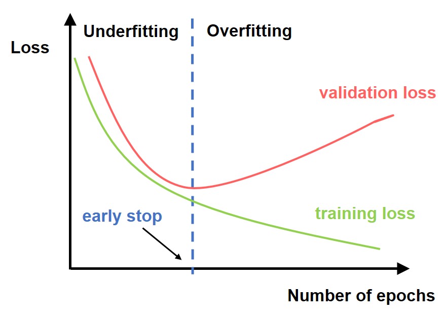
Graphical explanation of overfitting. Source: https://datahacker.rs/018-pytorch-popular-techniques-to-prevent-the-overfitting-in-a-neural-networks/.
# Track training and overfitting
# ==============================================================================
fig, ax = plt.subplots(figsize=(8, 3))
_ = forecaster.plot_history(ax=ax)

In the plot above, the training loss (blue) decreases rapidly during the first two epochs, indicating the model is quickly capturing the main patterns in the data. The validation loss (red) starts low and remains stable throughout the training process, closely following the training loss. This suggests:
The model is not overfitting, as the validation loss stays close to the training loss for all epochs.
Both losses decrease and stabilize together, indicating good generalization and effective learning.
No divergence is observed, which would appear as the validation loss increasing while training loss keeps decreasing.
# Predictions
# ==============================================================================
predictions = forecaster.predict()
predictions
| level | pred | |
|---|---|---|
| 2021-04-01 | o3 | 48.646408 |
In time series forecasting, the process of backtesting consists of evaluating the performance of a predictive model by applying it retrospectively to historical data. Therefore, it is a special type of cross-validation applied to the previous period(s). To learn more about backtesting, visit the backtesting user guide.
# Backtesting with test data
# ==============================================================================
cv = TimeSeriesFold(
         steps              = forecaster.max_step,
         initial_train_size = len(data.loc[:end_validation, :]),  # Training + Validation Data
         refit              = False
     )

metrics, predictions = backtesting_forecaster_multiseries(
    forecaster  = forecaster,
    series      = data[['o3']],
    cv          = cv,
    levels      = forecaster.levels,
    metric      = "mean_absolute_error",
    verbose     = False  # Set to True for detailed output
)
Epoch 1/25
48/48 ━━━━━━━━━━━━━━━━━━━━ 3s 39ms/step - loss: 0.0054 - val_loss: 0.0056
Epoch 2/25
48/48 ━━━━━━━━━━━━━━━━━━━━ 2s 39ms/step - loss: 0.0052 - val_loss: 0.0054
Epoch 3/25
48/48 ━━━━━━━━━━━━━━━━━━━━ 2s 37ms/step - loss: 0.0053 - val_loss: 0.0053
Epoch 4/25
48/48 ━━━━━━━━━━━━━━━━━━━━ 2s 34ms/step - loss: 0.0052 - val_loss: 0.0053
Epoch 5/25
48/48 ━━━━━━━━━━━━━━━━━━━━ 2s 41ms/step - loss: 0.0052 - val_loss: 0.0053
Epoch 6/25
48/48 ━━━━━━━━━━━━━━━━━━━━ 2s 33ms/step - loss: 0.0052 - val_loss: 0.0052
Epoch 7/25
48/48 ━━━━━━━━━━━━━━━━━━━━ 2s 32ms/step - loss: 0.0052 - val_loss: 0.0055
Epoch 8/25
48/48 ━━━━━━━━━━━━━━━━━━━━ 2s 33ms/step - loss: 0.0051 - val_loss: 0.0055
Epoch 9/25
48/48 ━━━━━━━━━━━━━━━━━━━━ 2s 31ms/step - loss: 0.0051 - val_loss: 0.0050
Epoch 10/25
48/48 ━━━━━━━━━━━━━━━━━━━━ 1s 31ms/step - loss: 0.0050 - val_loss: 0.0055
Epoch 11/25
48/48 ━━━━━━━━━━━━━━━━━━━━ 2s 34ms/step - loss: 0.0049 - val_loss: 0.0050
Epoch 12/25
48/48 ━━━━━━━━━━━━━━━━━━━━ 1s 30ms/step - loss: 0.0049 - val_loss: 0.0050
Epoch 13/25
48/48 ━━━━━━━━━━━━━━━━━━━━ 2s 32ms/step - loss: 0.0050 - val_loss: 0.0048
Epoch 14/25
48/48 ━━━━━━━━━━━━━━━━━━━━ 2s 32ms/step - loss: 0.0050 - val_loss: 0.0048
Epoch 15/25
48/48 ━━━━━━━━━━━━━━━━━━━━ 1s 30ms/step - loss: 0.0048 - val_loss: 0.0053
Epoch 16/25
48/48 ━━━━━━━━━━━━━━━━━━━━ 2s 32ms/step - loss: 0.0050 - val_loss: 0.0057
Epoch 17/25
48/48 ━━━━━━━━━━━━━━━━━━━━ 2s 34ms/step - loss: 0.0051 - val_loss: 0.0051
0%| | 0/2208 [00:00<?, ?it/s]
# Backtesting metrics
# ==============================================================================
metrics
| levels | mean_absolute_error | |
|---|---|---|
| 0 | o3 | 5.745553 |
# Backtesting predictions
# ==============================================================================
predictions.head(4)
| level | pred | |
|---|---|---|
| 2021-10-01 00:00:00 | o3 | 52.571770 |
| 2021-10-01 01:00:00 | o3 | 56.919910 |
| 2021-10-01 02:00:00 | o3 | 60.340588 |
| 2021-10-01 03:00:00 | o3 | 60.829491 |
# Plotting predictions vs real values in the test set
# ==============================================================================
fig, ax = plt.subplots(figsize=(8, 3))
data_test["o3"].plot(ax=ax, label="test")
predictions.loc[predictions["level"] == "o3", "pred"].plot(ax=ax, label="predictions")
ax.set_title("O3")
ax.legend();

2. Single-Series, Multi-Step Forecasting (1:1, Multiple Steps)
In this scenario, the objective is to predict multiple future values of a single time series using only its own past observations as predictors. This is known as multi-step univariate forecasting.
For example: Given a sequence of values ${y_{t-24}, ..., y_{t-1}}$, predict ${y_{t+1}, y_{t+2}, ..., y_{t+n}}$, where $n$ is the prediction horizon (number of steps ahead).
This setup is common when you want to forecast several periods into the future (e.g., the next 24 hours of ozone concentration).
Model Architecture
You can use a similar network architecture as in the single-step case, but predicting multiple steps ahead usually benefits from increasing the capacity of the model (e.g., more units in LSTM/GRU layers or additional dense layers). This allows the model to better capture the complexity of forecasting several points at once.
# Create model
# ==============================================================================
lags = 24

model = create_and_compile_model(
    series                  = data[["o3"]],  # Only the 'o3' series is used as predictor
    levels                  = ["o3"],        # Target series to predict
    lags                    = lags,          # Number of lags to use as predictors
    steps                   = 24,            # Multi-step forecasting
    recurrent_layer         = "GRU",
    recurrent_units         = 128,
    recurrent_layers_kwargs = {"activation": "tanh"},
    dense_units             = 64,
    compile_kwargs          = {'optimizer': 'adam', 'loss': 'mse'},
    model_name              = "Single-Series-Multi-Step"
)

model.summary()
keras version: 3.10.0
Using backend: tensorflow
tensorflow version: 2.19.0
Model: "Single-Series-Multi-Step"
┏━━━━━━━━━━━━━━━━━━━━━━━━━━━━━━━━━┳━━━━━━━━━━━━━━━━━━━━━━━━┳━━━━━━━━━━━━━━━┓
┃ Layer (type)                    ┃ Output Shape           ┃       Param # ┃
┡━━━━━━━━━━━━━━━━━━━━━━━━━━━━━━━━━╇━━━━━━━━━━━━━━━━━━━━━━━━╇━━━━━━━━━━━━━━━┩
│ series_input (InputLayer)       │ (None, 24, 1)          │             0 │
├─────────────────────────────────┼────────────────────────┼───────────────┤
│ gru_1 (GRU)                     │ (None, 128)            │        50,304 │
├─────────────────────────────────┼────────────────────────┼───────────────┤
│ dense_1 (Dense)                 │ (None, 64)             │         8,256 │
├─────────────────────────────────┼────────────────────────┼───────────────┤
│ output_dense_td_layer (Dense)   │ (None, 24)             │         1,560 │
├─────────────────────────────────┼────────────────────────┼───────────────┤
│ reshape (Reshape)               │ (None, 24, 1)          │             0 │
└─────────────────────────────────┴────────────────────────┴───────────────┘
Total params: 60,120 (234.84 KB)
Trainable params: 60,120 (234.84 KB)
Non-trainable params: 0 (0.00 B)
✎ Note
The fit_kwargs parameter lets you customize any aspect of the model training process, passing arguments directly to the underlying Keras Model.fit() method. For example, you can specify the number of training epochs, batch size, and any callbacks you want to use.
In the code example, the model is trained for 50 epochs with a batch size of 512. The EarlyStopping callback monitors the validation loss and automatically stops training if it does not improve for 3 consecutive epochs (patience=3). This helps prevent overfitting and saves computation time.
You can also add other callbacks, such as ModelCheckpoint to save the model at each epoch, or TensorBoard for real-time visualization of training and validation metrics.
# Forecaster Creation
# ==============================================================================
forecaster = ForecasterRnn(
    regressor=model,
    levels=["o3"],
    lags=lags,
    transformer_series=MinMaxScaler(),
    fit_kwargs={
        "epochs": 25,
        "batch_size": 512,
        "callbacks": [
            EarlyStopping(monitor="val_loss", patience=3, restore_best_weights=True)
        ],  # Callback to stop training when it is no longer learning.
        "series_val": data_val,  # Validation data for model training.
    },
)

# Fit forecaster
# ==============================================================================
forecaster.fit(data_train[['o3']])
Epoch 1/25
c:\Users\jaesc2\Miniconda3\envs\skforecast_py12\Lib\site-packages\keras\src\saving\saving_lib.py:802: UserWarning: Skipping variable loading for optimizer 'adam', because it has 16 variables whereas the saved optimizer has 2 variables.
  saveable.load_own_variables(weights_store.get(inner_path))
39/39 ━━━━━━━━━━━━━━━━━━━━ 3s 62ms/step - loss: 0.1136 - val_loss: 0.0312
Epoch 2/25
39/39 ━━━━━━━━━━━━━━━━━━━━ 2s 60ms/step - loss: 0.0297 - val_loss: 0.0263
Epoch 3/25
39/39 ━━━━━━━━━━━━━━━━━━━━ 2s 61ms/step - loss: 0.0265 - val_loss: 0.0237
Epoch 4/25
39/39 ━━━━━━━━━━━━━━━━━━━━ 2s 58ms/step - loss: 0.0243 - val_loss: 0.0206
Epoch 5/25
39/39 ━━━━━━━━━━━━━━━━━━━━ 2s 57ms/step - loss: 0.0218 - val_loss: 0.0184
Epoch 6/25
39/39 ━━━━━━━━━━━━━━━━━━━━ 2s 57ms/step - loss: 0.0205 - val_loss: 0.0183
Epoch 7/25
39/39 ━━━━━━━━━━━━━━━━━━━━ 2s 57ms/step - loss: 0.0201 - val_loss: 0.0175
Epoch 8/25
39/39 ━━━━━━━━━━━━━━━━━━━━ 2s 57ms/step - loss: 0.0198 - val_loss: 0.0170
Epoch 9/25
39/39 ━━━━━━━━━━━━━━━━━━━━ 2s 58ms/step - loss: 0.0193 - val_loss: 0.0168
Epoch 10/25
39/39 ━━━━━━━━━━━━━━━━━━━━ 2s 58ms/step - loss: 0.0191 - val_loss: 0.0167
Epoch 11/25
39/39 ━━━━━━━━━━━━━━━━━━━━ 2s 58ms/step - loss: 0.0189 - val_loss: 0.0167
Epoch 12/25
39/39 ━━━━━━━━━━━━━━━━━━━━ 2s 58ms/step - loss: 0.0186 - val_loss: 0.0166
Epoch 13/25
39/39 ━━━━━━━━━━━━━━━━━━━━ 2s 57ms/step - loss: 0.0185 - val_loss: 0.0165
Epoch 14/25
39/39 ━━━━━━━━━━━━━━━━━━━━ 2s 57ms/step - loss: 0.0184 - val_loss: 0.0165
Epoch 15/25
39/39 ━━━━━━━━━━━━━━━━━━━━ 2s 58ms/step - loss: 0.0182 - val_loss: 0.0173
Epoch 16/25
39/39 ━━━━━━━━━━━━━━━━━━━━ 2s 57ms/step - loss: 0.0182 - val_loss: 0.0163
Epoch 17/25
39/39 ━━━━━━━━━━━━━━━━━━━━ 2s 59ms/step - loss: 0.0177 - val_loss: 0.0165
Epoch 18/25
39/39 ━━━━━━━━━━━━━━━━━━━━ 2s 57ms/step - loss: 0.0177 - val_loss: 0.0163
Epoch 19/25
39/39 ━━━━━━━━━━━━━━━━━━━━ 2s 57ms/step - loss: 0.0176 - val_loss: 0.0161
Epoch 20/25
39/39 ━━━━━━━━━━━━━━━━━━━━ 2s 57ms/step - loss: 0.0177 - val_loss: 0.0162
Epoch 21/25
39/39 ━━━━━━━━━━━━━━━━━━━━ 2s 58ms/step - loss: 0.0175 - val_loss: 0.0166
Epoch 22/25
39/39 ━━━━━━━━━━━━━━━━━━━━ 2s 59ms/step - loss: 0.0173 - val_loss: 0.0160
Epoch 23/25
39/39 ━━━━━━━━━━━━━━━━━━━━ 2s 57ms/step - loss: 0.0172 - val_loss: 0.0164
Epoch 24/25
39/39 ━━━━━━━━━━━━━━━━━━━━ 2s 58ms/step - loss: 0.0172 - val_loss: 0.0160
Epoch 25/25
39/39 ━━━━━━━━━━━━━━━━━━━━ 2s 58ms/step - loss: 0.0173 - val_loss: 0.0160
# Train and overfitting tracking
# ==============================================================================
fig, ax = plt.subplots(figsize=(8, 3))
_ = forecaster.plot_history(ax=ax)

In this case, the prediction quality is expected to be lower than in the previous example, as shown by the higher loss values across epochs. This is easily explained: the model now has to predict 24 values at each step instead of just 1. As a result, the validation loss is higher, since it reflects the combined error across all 24 predicted values, rather than the error for a single value.
# Prediction
# ==============================================================================
predictions = forecaster.predict()
predictions.head(4)
| level | pred | |
|---|---|---|
| 2021-04-01 00:00:00 | o3 | 48.992241 |
| 2021-04-01 01:00:00 | o3 | 45.452671 |
| 2021-04-01 02:00:00 | o3 | 40.783764 |
| 2021-04-01 03:00:00 | o3 | 39.934483 |
# Specific step predictions
# ==============================================================================
predictions = forecaster.predict(steps=[1, 3])
predictions
| level | pred | |
|---|---|---|
| 2021-04-01 00:00:00 | o3 | 48.992241 |
| 2021-04-01 02:00:00 | o3 | 40.783764 |
# Backtesting
# ==============================================================================
cv = TimeSeriesFold(
         steps              = forecaster.max_step,
         initial_train_size = len(data.loc[:end_validation, :]),  # Training + Validation Data
         refit              = False
     )

metrics, predictions = backtesting_forecaster_multiseries(
    forecaster        = forecaster,
    series            = data[['o3']],
    cv                = cv,
    levels            = forecaster.levels,
    metric            = "mean_absolute_error",
    verbose           = False,
    suppress_warnings = True
)
Epoch 1/25
47/47 ━━━━━━━━━━━━━━━━━━━━ 4s 62ms/step - loss: 0.0169 - val_loss: 0.0158
Epoch 2/25
47/47 ━━━━━━━━━━━━━━━━━━━━ 3s 58ms/step - loss: 0.0170 - val_loss: 0.0157
Epoch 3/25
47/47 ━━━━━━━━━━━━━━━━━━━━ 3s 56ms/step - loss: 0.0168 - val_loss: 0.0158
Epoch 4/25
47/47 ━━━━━━━━━━━━━━━━━━━━ 3s 58ms/step - loss: 0.0167 - val_loss: 0.0158
Epoch 5/25
47/47 ━━━━━━━━━━━━━━━━━━━━ 3s 56ms/step - loss: 0.0165 - val_loss: 0.0160
0%| | 0/92 [00:00<?, ?it/s]
# Backtesting metrics
# ==============================================================================
metric_single_series = metrics.loc[metrics["levels"] == "o3", "mean_absolute_error"].iat[0]
metrics
| levels | mean_absolute_error | |
|---|---|---|
| 0 | o3 | 11.271916 |
# Backtesting predictions
# ==============================================================================
predictions
| level | pred | |
|---|---|---|
| 2021-10-01 00:00:00 | o3 | 60.107918 |
| 2021-10-01 01:00:00 | o3 | 58.672436 |
| 2021-10-01 02:00:00 | o3 | 54.720192 |
| 2021-10-01 03:00:00 | o3 | 50.960598 |
| 2021-10-01 04:00:00 | o3 | 46.120068 |
| ... | ... | ... |
| 2021-12-31 19:00:00 | o3 | 16.421032 |
| 2021-12-31 20:00:00 | o3 | 17.846300 |
| 2021-12-31 21:00:00 | o3 | 21.751144 |
| 2021-12-31 22:00:00 | o3 | 24.250710 |
| 2021-12-31 23:00:00 | o3 | 26.225739 |
2208 rows × 2 columns
# Plotting predictions vs real values in the test set
# ==============================================================================
fig, ax = plt.subplots(figsize=(8, 3))
data_test["o3"].plot(ax=ax, label="test")
predictions.loc[predictions["level"] == "o3", "pred"].plot(ax=ax, label="predictions")
ax.set_title("O3")
ax.legend();

3. Multi-Series, Single-Output Forecasting (N:1, Multiple Steps)
In this scenario, the goal is to predict future values of a single target time series by leveraging the past values of multiple related series as predictors. This is known as multivariate forecasting, where the model uses the historical data from several variables to improve the prediction of one specific series.
For example: Suppose you want to forecast ozone concentration (o3) for the next 24 hours. In addition to past o3 values, you may include other series—such as temperature, wind speed, or other pollutant concentrations—as predictors. The model will then use the combined information from all available series to make a more accurate forecast.
Model setup
To handle this type of problem, the neural network architecture becomes a bit more complex. An additional recurrent layer is used to process the information from multiple input series, and another dense (fully connected) layer further processes the output from the recurrent layer. With skforecast, building such a model is straightforward: simply pass a list of integers to the recurrent_units and dense_units arguments to add multiple recurrent and dense layers as needed.
# Create model
# ==============================================================================
lags = 24

model = create_and_compile_model(
    series                  = data,    # DataFrame with all series (predictors)
    levels                  = ["o3"],  # Target series to predict
    lags                    = lags,    # Number of lags to use as predictors
    steps                   = 24,      # Multi-step forecasting
    recurrent_layer         = "GRU",
    recurrent_units         = [128, 64],
    recurrent_layers_kwargs = {"activation": "tanh"},
    dense_units             = [64, 32],
    compile_kwargs          = {'optimizer': 'adam', 'loss': 'mse'},
    model_name              = "MultiVariate-Multi-Step"
)

model.summary()
keras version: 3.10.0
Using backend: tensorflow
tensorflow version: 2.19.0
Model: "MultiVariate-Multi-Step"
┏━━━━━━━━━━━━━━━━━━━━━━━━━━━━━━━━━┳━━━━━━━━━━━━━━━━━━━━━━━━┳━━━━━━━━━━━━━━━┓
┃ Layer (type)                    ┃ Output Shape           ┃       Param # ┃
┡━━━━━━━━━━━━━━━━━━━━━━━━━━━━━━━━━╇━━━━━━━━━━━━━━━━━━━━━━━━╇━━━━━━━━━━━━━━━┩
│ series_input (InputLayer)       │ (None, 24, 10)         │             0 │
├─────────────────────────────────┼────────────────────────┼───────────────┤
│ gru_1 (GRU)                     │ (None, 24, 128)        │        53,760 │
├─────────────────────────────────┼────────────────────────┼───────────────┤
│ gru_2 (GRU)                     │ (None, 64)             │        37,248 │
├─────────────────────────────────┼────────────────────────┼───────────────┤
│ dense_1 (Dense)                 │ (None, 64)             │         4,160 │
├─────────────────────────────────┼────────────────────────┼───────────────┤
│ dense_2 (Dense)                 │ (None, 32)             │         2,080 │
├─────────────────────────────────┼────────────────────────┼───────────────┤
│ output_dense_td_layer (Dense)   │ (None, 24)             │           792 │
├─────────────────────────────────┼────────────────────────┼───────────────┤
│ reshape (Reshape)               │ (None, 24, 1)          │             0 │
└─────────────────────────────────┴────────────────────────┴───────────────┘
Total params: 98,040 (382.97 KB)
Trainable params: 98,040 (382.97 KB)
Non-trainable params: 0 (0.00 B)
# Forecaster Creation
# ==============================================================================
forecaster = ForecasterRnn(
    regressor=model,
    levels=["o3"],
    lags=lags,
    transformer_series=MinMaxScaler(),
    fit_kwargs={
        "epochs": 25,
        "batch_size": 512,
        "callbacks": [
            EarlyStopping(monitor="val_loss", patience=3, restore_best_weights=True)
        ],  # Callback to stop training when it is no longer learning.
        "series_val": data_val,  # Validation data for model training.
    },
)

# Fit forecaster
# ==============================================================================
forecaster.fit(data_train)
c:\Users\jaesc2\Miniconda3\envs\skforecast_py12\Lib\site-packages\keras\src\saving\saving_lib.py:802: UserWarning: Skipping variable loading for optimizer 'adam', because it has 26 variables whereas the saved optimizer has 2 variables.
  saveable.load_own_variables(weights_store.get(inner_path))
Epoch 1/25
39/39 ━━━━━━━━━━━━━━━━━━━━ 5s 100ms/step - loss: 0.1185 - val_loss: 0.0470
Epoch 2/25
39/39 ━━━━━━━━━━━━━━━━━━━━ 4s 92ms/step - loss: 0.0356 - val_loss: 0.0288
Epoch 3/25
39/39 ━━━━━━━━━━━━━━━━━━━━ 4s 94ms/step - loss: 0.0276 - val_loss: 0.0264
Epoch 4/25
39/39 ━━━━━━━━━━━━━━━━━━━━ 4s 92ms/step - loss: 0.0264 - val_loss: 0.0251
Epoch 5/25
39/39 ━━━━━━━━━━━━━━━━━━━━ 4s 93ms/step - loss: 0.0252 - val_loss: 0.0224
Epoch 6/25
39/39 ━━━━━━━━━━━━━━━━━━━━ 4s 92ms/step - loss: 0.0227 - val_loss: 0.0193
Epoch 7/25
39/39 ━━━━━━━━━━━━━━━━━━━━ 4s 92ms/step - loss: 0.0206 - val_loss: 0.0173
Epoch 8/25
39/39 ━━━━━━━━━━━━━━━━━━━━ 4s 92ms/step - loss: 0.0191 - val_loss: 0.0163
Epoch 9/25
39/39 ━━━━━━━━━━━━━━━━━━━━ 4s 107ms/step - loss: 0.0180 - val_loss: 0.0161
Epoch 10/25
39/39 ━━━━━━━━━━━━━━━━━━━━ 4s 107ms/step - loss: 0.0175 - val_loss: 0.0157
Epoch 11/25
39/39 ━━━━━━━━━━━━━━━━━━━━ 4s 107ms/step - loss: 0.0171 - val_loss: 0.0158
Epoch 12/25
39/39 ━━━━━━━━━━━━━━━━━━━━ 4s 105ms/step - loss: 0.0167 - val_loss: 0.0161
Epoch 13/25
39/39 ━━━━━━━━━━━━━━━━━━━━ 4s 107ms/step - loss: 0.0165 - val_loss: 0.0151
Epoch 14/25
39/39 ━━━━━━━━━━━━━━━━━━━━ 4s 106ms/step - loss: 0.0163 - val_loss: 0.0151
Epoch 15/25
39/39 ━━━━━━━━━━━━━━━━━━━━ 4s 107ms/step - loss: 0.0160 - val_loss: 0.0152
Epoch 16/25
39/39 ━━━━━━━━━━━━━━━━━━━━ 4s 105ms/step - loss: 0.0160 - val_loss: 0.0150
Epoch 17/25
39/39 ━━━━━━━━━━━━━━━━━━━━ 4s 106ms/step - loss: 0.0156 - val_loss: 0.0149
Epoch 18/25
39/39 ━━━━━━━━━━━━━━━━━━━━ 4s 105ms/step - loss: 0.0158 - val_loss: 0.0153
Epoch 19/25
39/39 ━━━━━━━━━━━━━━━━━━━━ 4s 106ms/step - loss: 0.0155 - val_loss: 0.0150
Epoch 20/25
39/39 ━━━━━━━━━━━━━━━━━━━━ 4s 112ms/step - loss: 0.0153 - val_loss: 0.0150
# Training and overfitting tracking
# ==============================================================================
fig, ax = plt.subplots(figsize=(8, 3))
_ = forecaster.plot_history(ax=ax)

# Prediction
# ==============================================================================
predictions = forecaster.predict()
predictions.head(4)
| level | pred | |
|---|---|---|
| 2021-04-01 00:00:00 | o3 | 52.557709 |
| 2021-04-01 01:00:00 | o3 | 51.103519 |
| 2021-04-01 02:00:00 | o3 | 47.209839 |
| 2021-04-01 03:00:00 | o3 | 43.603031 |
# Backtesting with test data
# ==============================================================================
cv = TimeSeriesFold(
         steps              = forecaster.max_step,
         initial_train_size = len(data.loc[:end_validation, :]),  # Training + Validation Data
         refit              = False
     )

metrics, predictions = backtesting_forecaster_multiseries(
    forecaster        = forecaster,
    series            = data,
    cv                = cv,
    levels            = forecaster.levels,
    metric            = "mean_absolute_error",
    suppress_warnings = True,
    verbose           = False
)
Epoch 1/25
47/47 ━━━━━━━━━━━━━━━━━━━━ 7s 114ms/step - loss: 0.0155 - val_loss: 0.0147
Epoch 2/25
47/47 ━━━━━━━━━━━━━━━━━━━━ 5s 104ms/step - loss: 0.0153 - val_loss: 0.0145
Epoch 3/25
47/47 ━━━━━━━━━━━━━━━━━━━━ 5s 105ms/step - loss: 0.0151 - val_loss: 0.0143
Epoch 4/25
47/47 ━━━━━━━━━━━━━━━━━━━━ 5s 106ms/step - loss: 0.0150 - val_loss: 0.0143
Epoch 5/25
47/47 ━━━━━━━━━━━━━━━━━━━━ 5s 104ms/step - loss: 0.0147 - val_loss: 0.0140
Epoch 6/25
47/47 ━━━━━━━━━━━━━━━━━━━━ 5s 103ms/step - loss: 0.0148 - val_loss: 0.0141
Epoch 7/25
47/47 ━━━━━━━━━━━━━━━━━━━━ 5s 105ms/step - loss: 0.0148 - val_loss: 0.0139
Epoch 8/25
47/47 ━━━━━━━━━━━━━━━━━━━━ 5s 102ms/step - loss: 0.0147 - val_loss: 0.0138
Epoch 9/25
47/47 ━━━━━━━━━━━━━━━━━━━━ 5s 104ms/step - loss: 0.0146 - val_loss: 0.0138
Epoch 10/25
47/47 ━━━━━━━━━━━━━━━━━━━━ 5s 104ms/step - loss: 0.0143 - val_loss: 0.0138
Epoch 11/25
47/47 ━━━━━━━━━━━━━━━━━━━━ 5s 102ms/step - loss: 0.0143 - val_loss: 0.0139
Epoch 12/25
47/47 ━━━━━━━━━━━━━━━━━━━━ 5s 103ms/step - loss: 0.0143 - val_loss: 0.0138
Epoch 13/25
47/47 ━━━━━━━━━━━━━━━━━━━━ 5s 102ms/step - loss: 0.0142 - val_loss: 0.0138
0%| | 0/92 [00:00<?, ?it/s]
# Backtesting metrics
# ==============================================================================
metric_multivariate = metrics.loc[metrics["levels"] == "o3", "mean_absolute_error"].iat[0]
metrics
| levels | mean_absolute_error | |
|---|---|---|
| 0 | o3 | 10.90494 |
# Backtesting predictions
# ==============================================================================
predictions
| level | pred | |
|---|---|---|
| 2021-10-01 00:00:00 | o3 | 51.411842 |
| 2021-10-01 01:00:00 | o3 | 50.147354 |
| 2021-10-01 02:00:00 | o3 | 46.690861 |
| 2021-10-01 03:00:00 | o3 | 40.983303 |
| 2021-10-01 04:00:00 | o3 | 37.137405 |
| ... | ... | ... |
| 2021-12-31 19:00:00 | o3 | 21.922625 |
| 2021-12-31 20:00:00 | o3 | 20.657047 |
| 2021-12-31 21:00:00 | o3 | 17.817327 |
| 2021-12-31 22:00:00 | o3 | 15.759877 |
| 2021-12-31 23:00:00 | o3 | 15.729614 |
2208 rows × 2 columns
# Plotting predictions vs real values in the test set
# ==============================================================================
fig, ax = plt.subplots(figsize=(8, 3))
data_test["o3"].plot(ax=ax, label="test")
predictions.loc[predictions["level"] == "o3", "pred"].plot(ax=ax, label="predictions")
ax.set_title("O3")
ax.legend()
plt.show()

When using multiple time series as predictors, it is often expected that the model will produce more accurate forecasts for the target series. However, in this example, the predictions are actually worse than in the previous case where only a single series was used as input. This may happen if the additional time series used as predictors are not strongly related to the target series. As a result, the model is unable to learn meaningful relationships, and the extra information does not improve performance—in fact, it may even introduce noise.
4. Multi-Series, Multi-Output Forecasting (N:M, Multiple Steps)
In this scenario, the goal is to predict multiple future values for several time series at once, using the historical data from all available series as input. This is known as multivariate-multioutput forecasting.
With this approach, a single model learns to predict several target series simultaneously, capturing relationships and dependencies not only within each series, but also across different series.
Real-world applications include:
Forecasting the sales of multiple products in an online store, leveraging past sales, pricing history, promotions, and other product-related variables.
Study the flue gas emissions of a gas turbine, where you want to predict the concentration of multiple pollutants (e.g., NOX, CO) based on past emissions data and other related variables.
Modeling environmental variables (e.g., pollution, temperature, humidity) together, where the evolution of one variable may influence or be influenced by others.
# Create model
# ==============================================================================
levels = ['o3', 'pm2.5', 'pm10']  # Multiple target series to predict
lags = 24

model = create_and_compile_model(
    series                  = data,    # DataFrame with all series (predictors)
    levels                  = levels,
    lags                    = lags,
    steps                   = 24,
    recurrent_layer         = "LSTM",
    recurrent_units         = [128, 64],
    recurrent_layers_kwargs = {"activation": "tanh"},
    dense_units             = [64, 32],
    compile_kwargs          = {'optimizer': Adam(), 'loss': MeanSquaredError()},
    model_name              = "MultiVariate-MultiOutput-Multi-Step"
)

model.summary()
keras version: 3.10.0
Using backend: tensorflow
tensorflow version: 2.19.0
Model: "MultiVariate-MultiOutput-Multi-Step"
┏━━━━━━━━━━━━━━━━━━━━━━━━━━━━━━━━━┳━━━━━━━━━━━━━━━━━━━━━━━━┳━━━━━━━━━━━━━━━┓
┃ Layer (type)                    ┃ Output Shape           ┃       Param # ┃
┡━━━━━━━━━━━━━━━━━━━━━━━━━━━━━━━━━╇━━━━━━━━━━━━━━━━━━━━━━━━╇━━━━━━━━━━━━━━━┩
│ series_input (InputLayer)       │ (None, 24, 10)         │             0 │
├─────────────────────────────────┼────────────────────────┼───────────────┤
│ lstm_1 (LSTM)                   │ (None, 24, 128)        │        71,168 │
├─────────────────────────────────┼────────────────────────┼───────────────┤
│ lstm_2 (LSTM)                   │ (None, 64)             │        49,408 │
├─────────────────────────────────┼────────────────────────┼───────────────┤
│ dense_1 (Dense)                 │ (None, 64)             │         4,160 │
├─────────────────────────────────┼────────────────────────┼───────────────┤
│ dense_2 (Dense)                 │ (None, 32)             │         2,080 │
├─────────────────────────────────┼────────────────────────┼───────────────┤
│ output_dense_td_layer (Dense)   │ (None, 72)             │         2,376 │
├─────────────────────────────────┼────────────────────────┼───────────────┤
│ reshape (Reshape)               │ (None, 24, 3)          │             0 │
└─────────────────────────────────┴────────────────────────┴───────────────┘
Total params: 129,192 (504.66 KB)
Trainable params: 129,192 (504.66 KB)
Non-trainable params: 0 (0.00 B)
# Forecaster Creation
# ==============================================================================
forecaster = ForecasterRnn(
    regressor=model,
    levels=levels,
    lags=lags,
    transformer_series=MinMaxScaler(),
    fit_kwargs={
        "epochs": 25,
        "batch_size": 512,
        "callbacks": [
            EarlyStopping(monitor="val_loss", patience=3, restore_best_weights=True)
        ],  # Callback to stop training when it is no longer learning.
        "series_val": data_val,  # Validation data for model training.
    },
)

# Fit forecaster
# ==============================================================================
forecaster.fit(data_train)
c:\Users\jaesc2\Miniconda3\envs\skforecast_py12\Lib\site-packages\keras\src\saving\saving_lib.py:802: UserWarning: Skipping variable loading for optimizer 'adam', because it has 26 variables whereas the saved optimizer has 2 variables.
  saveable.load_own_variables(weights_store.get(inner_path))
Epoch 1/25
39/39 ━━━━━━━━━━━━━━━━━━━━ 5s 90ms/step - loss: 0.0517 - val_loss: 0.0176
Epoch 2/25
39/39 ━━━━━━━━━━━━━━━━━━━━ 4s 93ms/step - loss: 0.0148 - val_loss: 0.0100
Epoch 3/25
39/39 ━━━━━━━━━━━━━━━━━━━━ 4s 96ms/step - loss: 0.0116 - val_loss: 0.0091
Epoch 4/25
39/39 ━━━━━━━━━━━━━━━━━━━━ 4s 101ms/step - loss: 0.0105 - val_loss: 0.0082
Epoch 5/25
39/39 ━━━━━━━━━━━━━━━━━━━━ 4s 103ms/step - loss: 0.0095 - val_loss: 0.0073
Epoch 6/25
39/39 ━━━━━━━━━━━━━━━━━━━━ 4s 100ms/step - loss: 0.0087 - val_loss: 0.0066
Epoch 7/25
39/39 ━━━━━━━━━━━━━━━━━━━━ 4s 98ms/step - loss: 0.0082 - val_loss: 0.0063
Epoch 8/25
39/39 ━━━━━━━━━━━━━━━━━━━━ 4s 98ms/step - loss: 0.0080 - val_loss: 0.0063
Epoch 9/25
39/39 ━━━━━━━━━━━━━━━━━━━━ 4s 93ms/step - loss: 0.0078 - val_loss: 0.0062
Epoch 10/25
39/39 ━━━━━━━━━━━━━━━━━━━━ 4s 97ms/step - loss: 0.0077 - val_loss: 0.0061
Epoch 11/25
39/39 ━━━━━━━━━━━━━━━━━━━━ 4s 100ms/step - loss: 0.0075 - val_loss: 0.0060
Epoch 12/25
39/39 ━━━━━━━━━━━━━━━━━━━━ 4s 95ms/step - loss: 0.0073 - val_loss: 0.0061
Epoch 13/25
39/39 ━━━━━━━━━━━━━━━━━━━━ 4s 94ms/step - loss: 0.0073 - val_loss: 0.0060
Epoch 14/25
39/39 ━━━━━━━━━━━━━━━━━━━━ 4s 94ms/step - loss: 0.0072 - val_loss: 0.0061
# Training and overfitting tracking
# ==============================================================================
fig, ax = plt.subplots(figsize=(8, 3))
_ = forecaster.plot_history(ax=ax)

Predictions can be made for specific steps and levels as long as they are within the prediction horizon defined by the model. For example, you can predict ozone concentration (levels = "o3") for the next one and five hours (steps = [1, 5]).
# Specific steps and levels predictions
# ==============================================================================
forecaster.predict(steps=[1, 5], levels="o3")
| level | pred | |
|---|---|---|
| 2021-04-01 00:00:00 | o3 | 51.330368 |
| 2021-04-01 04:00:00 | o3 | 33.898960 |
# Predictions for all steps and levels
# ==============================================================================
predictions = forecaster.predict()
predictions
| level | pred | |
|---|---|---|
| 2021-04-01 00:00:00 | o3 | 51.330368 |
| 2021-04-01 00:00:00 | pm2.5 | 13.790528 |
| 2021-04-01 00:00:00 | pm10 | 16.680853 |
| 2021-04-01 01:00:00 | o3 | 46.169151 |
| 2021-04-01 01:00:00 | pm2.5 | 14.281107 |
| ... | ... | ... |
| 2021-04-01 22:00:00 | pm2.5 | 11.015145 |
| 2021-04-01 22:00:00 | pm10 | 16.603825 |
| 2021-04-01 23:00:00 | o3 | 55.626831 |
| 2021-04-01 23:00:00 | pm2.5 | 11.014272 |
| 2021-04-01 23:00:00 | pm10 | 18.551624 |
72 rows × 2 columns
# Backtesting with test data
# ==============================================================================
cv = TimeSeriesFold(
         steps              = forecaster.max_step,
         initial_train_size = len(data.loc[:end_validation, :]),  # Training + Validation Data
         refit              = False
     )

metrics, predictions = backtesting_forecaster_multiseries(
    forecaster        = forecaster,
    series            = data,
    cv                = cv,
    levels            = forecaster.levels,
    metric            = "mean_absolute_error",
    suppress_warnings = True,
    verbose           = False
)
Epoch 1/25
47/47 ━━━━━━━━━━━━━━━━━━━━ 6s 100ms/step - loss: 0.0071 - val_loss: 0.0059
Epoch 2/25
47/47 ━━━━━━━━━━━━━━━━━━━━ 4s 93ms/step - loss: 0.0070 - val_loss: 0.0057
Epoch 3/25
47/47 ━━━━━━━━━━━━━━━━━━━━ 4s 93ms/step - loss: 0.0069 - val_loss: 0.0056
Epoch 4/25
47/47 ━━━━━━━━━━━━━━━━━━━━ 4s 93ms/step - loss: 0.0068 - val_loss: 0.0056
Epoch 5/25
47/47 ━━━━━━━━━━━━━━━━━━━━ 5s 95ms/step - loss: 0.0067 - val_loss: 0.0055
Epoch 6/25
47/47 ━━━━━━━━━━━━━━━━━━━━ 4s 93ms/step - loss: 0.0066 - val_loss: 0.0054
Epoch 7/25
47/47 ━━━━━━━━━━━━━━━━━━━━ 4s 93ms/step - loss: 0.0065 - val_loss: 0.0054
Epoch 8/25
47/47 ━━━━━━━━━━━━━━━━━━━━ 4s 94ms/step - loss: 0.0064 - val_loss: 0.0053
Epoch 9/25
47/47 ━━━━━━━━━━━━━━━━━━━━ 4s 93ms/step - loss: 0.0063 - val_loss: 0.0052
Epoch 10/25
47/47 ━━━━━━━━━━━━━━━━━━━━ 4s 95ms/step - loss: 0.0061 - val_loss: 0.0052
Epoch 11/25
47/47 ━━━━━━━━━━━━━━━━━━━━ 4s 94ms/step - loss: 0.0061 - val_loss: 0.0052
Epoch 12/25
47/47 ━━━━━━━━━━━━━━━━━━━━ 4s 94ms/step - loss: 0.0061 - val_loss: 0.0051
Epoch 13/25
47/47 ━━━━━━━━━━━━━━━━━━━━ 4s 94ms/step - loss: 0.0060 - val_loss: 0.0051
Epoch 14/25
47/47 ━━━━━━━━━━━━━━━━━━━━ 5s 95ms/step - loss: 0.0059 - val_loss: 0.0051
Epoch 15/25
47/47 ━━━━━━━━━━━━━━━━━━━━ 4s 94ms/step - loss: 0.0057 - val_loss: 0.0051
Epoch 16/25
47/47 ━━━━━━━━━━━━━━━━━━━━ 4s 93ms/step - loss: 0.0058 - val_loss: 0.0049
Epoch 17/25
47/47 ━━━━━━━━━━━━━━━━━━━━ 5s 96ms/step - loss: 0.0057 - val_loss: 0.0049
Epoch 18/25
47/47 ━━━━━━━━━━━━━━━━━━━━ 4s 95ms/step - loss: 0.0057 - val_loss: 0.0049
Epoch 19/25
47/47 ━━━━━━━━━━━━━━━━━━━━ 4s 95ms/step - loss: 0.0055 - val_loss: 0.0049
Epoch 20/25
47/47 ━━━━━━━━━━━━━━━━━━━━ 4s 92ms/step - loss: 0.0056 - val_loss: 0.0049
Epoch 21/25
47/47 ━━━━━━━━━━━━━━━━━━━━ 4s 93ms/step - loss: 0.0055 - val_loss: 0.0048
Epoch 22/25
47/47 ━━━━━━━━━━━━━━━━━━━━ 4s 95ms/step - loss: 0.0054 - val_loss: 0.0047
Epoch 23/25
47/47 ━━━━━━━━━━━━━━━━━━━━ 4s 94ms/step - loss: 0.0053 - val_loss: 0.0047
Epoch 24/25
47/47 ━━━━━━━━━━━━━━━━━━━━ 5s 101ms/step - loss: 0.0052 - val_loss: 0.0047
Epoch 25/25
47/47 ━━━━━━━━━━━━━━━━━━━━ 5s 97ms/step - loss: 0.0052 - val_loss: 0.0047
0%| | 0/92 [00:00<?, ?it/s]
# Backtesting metrics
# ==============================================================================
metric_multivariate_multioutput = metrics.loc[metrics["levels"] == "o3", "mean_absolute_error"].iat[0]
metrics
| levels | mean_absolute_error | |
|---|---|---|
| 0 | o3 | 11.682385 |
| 1 | pm2.5 | 4.018549 |
| 2 | pm10 | 12.209744 |
| 3 | average | 9.303559 |
| 4 | weighted_average | 9.303559 |
| 5 | pooling | 9.303559 |
# Plot all the predicted variables as rows in the plot
# ==============================================================================
fig, ax = plt.subplots(len(levels), 1, figsize=(8, 2 * len(levels)), sharex=True)
for i, level in enumerate(levels):
    data_test[level].plot(ax=ax[i], label="test")
    predictions.loc[predictions["level"] == level, "pred"].plot(ax=ax[i], label="predictions")
    ax[i].set_title(level)
    ax[i].legend()

plt.tight_layout()
plt.show()

Comparing Forecasting Strategies
As we have seen, various deep learning architectures and modeling strategies can be employed for time series forecasting. In summary, the forecasting approaches can be categorized into:
Single series, multi-step forecasting: Predict future values of a single series using only its past values.
Multivariate, single-output, multi-step forecasting: Use several series as predictors to forecast a target series over multiple future time steps.
Multivariate, multi-output, multi-step forecasting: Use multiple predictor series to forecast several targets over multiple steps.
Below is a summary table comparing the Mean Absolute Error (MAE) for each approach, calculated on the same target series, "o3":
# Metric comparison
# ==============================================================================
results = {
    "Single-Series, Multi-Step": metric_single_series,
    "Multi-Series, Single-Output": metric_multivariate,
    "Multi-Series, Multi-Output": metric_multivariate_multioutput
}

table_results = pd.DataFrame.from_dict(results, orient='index', columns=['O3 MAE'])
table_results = table_results.style.highlight_min(axis=0, color='green').format(precision=4)
table_results
| O3 MAE | |
|---|---|
| Single-Series, Multi-Step | 11.2719 |
| Multi-Series, Single-Output | 10.9049 |
| Multi-Series, Multi-Output | 11.6824 |
In this example, the single-series and simple multivariate approaches produce similar errors, while adding more targets as outputs (multi-output) increases the prediction error. However, there is no universal rule: the best strategy depends on your data, domain, and prediction goals.
It's important to experiment with different architectures and compare their metrics to select the most appropriate model for your specific use case.
Exogenous variables in deep learning models
Exogenous variables are external predictors (such as weather, holidays, or special events) that can influence the target series but are not part of its own historical values. When building deep learning models for time series forecasting, including these variables can help capture important patterns and improve accuracy, as long as their future values are available at prediction time.
In this section, we’ll demonstrate how to use exogenous variables in deep learning models with a new dataset: bike_sharing, which contains hourly bike usage in Washington D.C., together with weather and holiday information.
To learn more about exogenous variables in skforecast visit the exogenous variables user guide.
# Data download
# ==============================================================================
data_exog = fetch_dataset(name='bike_sharing', raw=False)
data_exog = data_exog[['users', 'temp', 'hum', 'windspeed', 'holiday']]
data_exog = data_exog.loc['2011-04-01 00:00:00':'2012-10-20 23:00:00', :].copy()
data_exog.head(3)
bike_sharing
------------
Hourly usage of the bike share system in the city of Washington D.C. during the
years 2011 and 2012. In addition to the number of users per hour, information
about weather conditions and holidays is available.
Fanaee-T,Hadi. (2013). Bike Sharing Dataset. UCI Machine Learning Repository.
https://doi.org/10.24432/C5W894.
Shape of the dataset: (17544, 11)
| users | temp | hum | windspeed | holiday | |
|---|---|---|---|---|---|
| date_time | |||||
| 2011-04-01 00:00:00 | 6.0 | 10.66 | 100.0 | 11.0014 | 0.0 |
| 2011-04-01 01:00:00 | 4.0 | 10.66 | 100.0 | 11.0014 | 0.0 |
| 2011-04-01 02:00:00 | 7.0 | 10.66 | 93.0 | 12.9980 | 0.0 |
# Calendar features
# ==============================================================================
features_to_extract = [
    'month',
    'week',
    'day_of_week',
    'hour'
]
calendar_transformer = DatetimeFeatures(
    variables           = 'index',
    features_to_extract = features_to_extract,
    drop_original       = False,
)

# Cyclical encoding of calendar features
# ==============================================================================
features_to_encode = [
    "month",
    "week",
    "day_of_week",
    "hour",
]
max_values = {
    "month": 12,
    "week": 52,
    "day_of_week": 7,
    "hour": 24,
}
cyclical_encoder = CyclicalFeatures(
                       variables     = features_to_encode,
                       max_values    = max_values,
                       drop_original = True
                   )

exog_transformer = make_pipeline(
                       calendar_transformer,
                       cyclical_encoder
                   )

data_exog = exog_transformer.fit_transform(data_exog)
exog_features = data_exog.columns.difference(['users']).tolist()

print(f"Exogenous features: {exog_features}")
data_exog.head(3)
Exogenous features: ['day_of_week_cos', 'day_of_week_sin', 'holiday', 'hour_cos', 'hour_sin', 'hum', 'month_cos', 'month_sin', 'temp', 'week_cos', 'week_sin', 'windspeed']
| users | temp | hum | windspeed | holiday | month_sin | month_cos | week_sin | week_cos | day_of_week_sin | day_of_week_cos | hour_sin | hour_cos | |
|---|---|---|---|---|---|---|---|---|---|---|---|---|---|
| date_time | |||||||||||||
| 2011-04-01 00:00:00 | 6.0 | 10.66 | 100.0 | 11.0014 | 0.0 | 0.866025 | -0.5 | 1.0 | 6.123234e-17 | -0.433884 | -0.900969 | 0.000000 | 1.000000 |
| 2011-04-01 01:00:00 | 4.0 | 10.66 | 100.0 | 11.0014 | 0.0 | 0.866025 | -0.5 | 1.0 | 6.123234e-17 | -0.433884 | -0.900969 | 0.258819 | 0.965926 |
| 2011-04-01 02:00:00 | 7.0 | 10.66 | 93.0 | 12.9980 | 0.0 | 0.866025 | -0.5 | 1.0 | 6.123234e-17 | -0.433884 | -0.900969 | 0.500000 | 0.866025 |
# Split train-validation-test
# ==============================================================================
end_train = '2012-06-30 23:59:00'
end_validation = '2012-10-01 23:59:00'
data_exog_train = data_exog.loc[: end_train, :]
data_exog_val   = data_exog.loc[end_train:end_validation, :]
data_exog_test  = data_exog.loc[end_validation:, :]

print(f"Dates train      : {data_exog_train.index.min()} --- {data_exog_train.index.max()}  (n={len(data_exog_train)})")
print(f"Dates validation : {data_exog_val.index.min()} --- {data_exog_val.index.max()}  (n={len(data_exog_val)})")
print(f"Dates test       : {data_exog_test.index.min()} --- {data_exog_test.index.max()}  (n={len(data_exog_test)})")
Dates train      : 2011-04-01 00:00:00 --- 2012-06-30 23:00:00  (n=10968)
Dates validation : 2012-07-01 00:00:00 --- 2012-10-01 23:00:00  (n=2232)
Dates test       : 2012-10-02 00:00:00 --- 2012-10-20 23:00:00  (n=456)
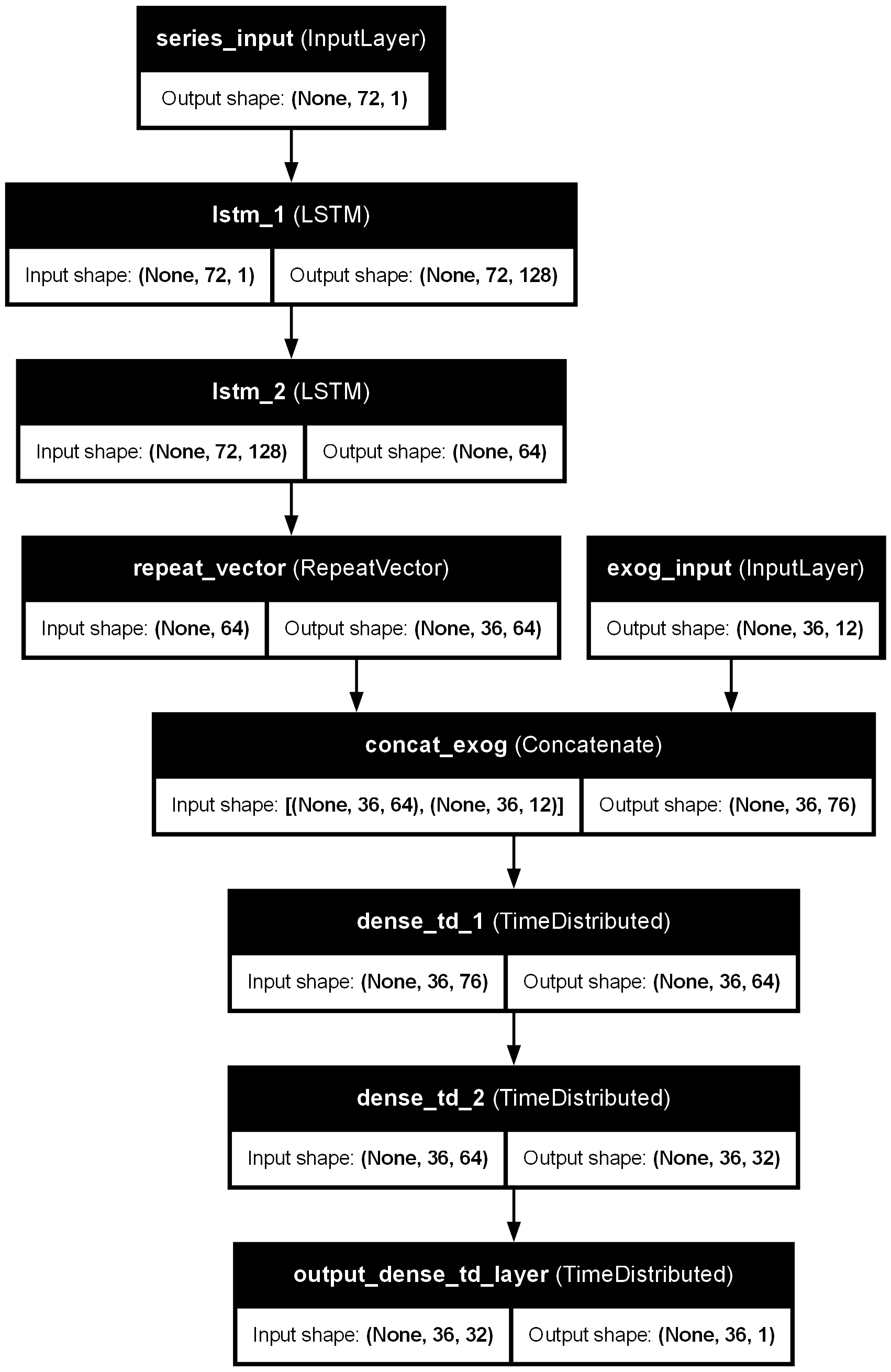
The architecture of your deep learning model must be able to accept extra inputs alongside the main time series data. The create_and_compile_model function makes this straightforward: simply pass the exogenous variables as a DataFrame to the exog argument.
# `create_and_compile_model` with exogenous variables
# ==============================================================================
series = ['users']
levels = ['users']
lags = 72

model = create_and_compile_model(
    series                  = data_exog[series],         # Single-series
    levels                  = levels,                    # One target series to predict
    lags                    = lags,
    steps                   = 36,
    exog                    = data_exog[exog_features],  # Exogenous variables
    recurrent_layer         = "LSTM",
    recurrent_units         = [128, 64],
    recurrent_layers_kwargs = {"activation": "tanh"},
    dense_units             = [64, 32],
    compile_kwargs          = {'optimizer': Adam(learning_rate=0.01), 'loss': 'mse'},
    model_name              = "Single-Series-Multi-Step-Exog"
)

model.summary()
keras version: 3.10.0
Using backend: tensorflow
tensorflow version: 2.19.0
Model: "Single-Series-Multi-Step-Exog"
┏━━━━━━━━━━━━━━━━━━━━━┳━━━━━━━━━━━━━━━━━━━┳━━━━━━━━━━━━┳━━━━━━━━━━━━━━━━━━━┓
┃ Layer (type)        ┃ Output Shape      ┃    Param # ┃ Connected to      ┃
┡━━━━━━━━━━━━━━━━━━━━━╇━━━━━━━━━━━━━━━━━━━╇━━━━━━━━━━━━╇━━━━━━━━━━━━━━━━━━━┩
│ series_input        │ (None, 72, 1)     │          0 │ -                 │
│ (InputLayer)        │                   │            │                   │
├─────────────────────┼───────────────────┼────────────┼───────────────────┤
│ lstm_1 (LSTM)       │ (None, 72, 128)   │     66,560 │ series_input[0][… │
├─────────────────────┼───────────────────┼────────────┼───────────────────┤
│ lstm_2 (LSTM)       │ (None, 64)        │     49,408 │ lstm_1[0][0]      │
├─────────────────────┼───────────────────┼────────────┼───────────────────┤
│ repeat_vector       │ (None, 36, 64)    │          0 │ lstm_2[0][0]      │
│ (RepeatVector)      │                   │            │                   │
├─────────────────────┼───────────────────┼────────────┼───────────────────┤
│ exog_input          │ (None, 36, 12)    │          0 │ -                 │
│ (InputLayer)        │                   │            │                   │
├─────────────────────┼───────────────────┼────────────┼───────────────────┤
│ concat_exog         │ (None, 36, 76)    │          0 │ repeat_vector[0]… │
│ (Concatenate)       │                   │            │ exog_input[0][0]  │
├─────────────────────┼───────────────────┼────────────┼───────────────────┤
│ dense_td_1          │ (None, 36, 64)    │      4,928 │ concat_exog[0][0] │
│ (TimeDistributed)   │                   │            │                   │
├─────────────────────┼───────────────────┼────────────┼───────────────────┤
│ dense_td_2          │ (None, 36, 32)    │      2,080 │ dense_td_1[0][0]  │
│ (TimeDistributed)   │                   │            │                   │
├─────────────────────┼───────────────────┼────────────┼───────────────────┤
│ output_dense_td_la… │ (None, 36, 1)     │         33 │ dense_td_2[0][0]  │
│ (TimeDistributed)   │                   │            │                   │
└─────────────────────┴───────────────────┴────────────┴───────────────────┘
Total params: 123,009 (480.50 KB)
Trainable params: 123,009 (480.50 KB)
Non-trainable params: 0 (0.00 B)
# Plotting the model architecture (require `pydot` and `graphviz`)
# ==============================================================================
# from keras.utils import plot_model
# plot_model(model, show_shapes=True, show_layer_names=True, to_file='model-architecture-exog.png')
# Forecaster Creation
# ==============================================================================
forecaster = ForecasterRnn(
    regressor=model,
    levels=levels,
    lags=lags,
    transformer_series=MinMaxScaler(),
    transformer_exog=MinMaxScaler(),
    fit_kwargs={
        "epochs": 25,
        "batch_size": 1024,
        "callbacks": [
            EarlyStopping(monitor="val_loss", patience=3, restore_best_weights=True),
            ReduceLROnPlateau(monitor="val_loss", factor=0.5, patience=2, min_lr=1e-5, verbose=1)
        ],  # Callback to stop training when it is no longer learning and to reduce learning rate.
        "series_val": data_exog_val[series],      # Validation data for model training.
        "exog_val": data_exog_val[exog_features]  # Validation data for exogenous variables
    },
)

# Fit forecaster with exogenous variables
# ==============================================================================
forecaster.fit(
    series = data_exog_train[series],
    exog   = data_exog_train[exog_features]
)
c:\Users\jaesc2\Miniconda3\envs\skforecast_py12\Lib\site-packages\keras\src\saving\saving_lib.py:802: UserWarning: Skipping variable loading for optimizer 'adam', because it has 26 variables whereas the saved optimizer has 2 variables.
  saveable.load_own_variables(weights_store.get(inner_path))
Epoch 1/25
11/11 ━━━━━━━━━━━━━━━━━━━━ 10s 650ms/step - loss: 0.1219 - val_loss: 0.0686 - learning_rate: 0.0100
Epoch 2/25
11/11 ━━━━━━━━━━━━━━━━━━━━ 7s 654ms/step - loss: 0.0240 - val_loss: 0.0448 - learning_rate: 0.0100
Epoch 3/25
11/11 ━━━━━━━━━━━━━━━━━━━━ 7s 643ms/step - loss: 0.0161 - val_loss: 0.0405 - learning_rate: 0.0100
Epoch 4/25
11/11 ━━━━━━━━━━━━━━━━━━━━ 7s 648ms/step - loss: 0.0144 - val_loss: 0.0360 - learning_rate: 0.0100
Epoch 5/25
11/11 ━━━━━━━━━━━━━━━━━━━━ 7s 654ms/step - loss: 0.0131 - val_loss: 0.0312 - learning_rate: 0.0100
Epoch 6/25
11/11 ━━━━━━━━━━━━━━━━━━━━ 7s 652ms/step - loss: 0.0118 - val_loss: 0.0305 - learning_rate: 0.0100
Epoch 7/25
11/11 ━━━━━━━━━━━━━━━━━━━━ 8s 691ms/step - loss: 0.0104 - val_loss: 0.0291 - learning_rate: 0.0100
Epoch 8/25
11/11 ━━━━━━━━━━━━━━━━━━━━ 8s 685ms/step - loss: 0.0096 - val_loss: 0.0270 - learning_rate: 0.0100
Epoch 9/25
11/11 ━━━━━━━━━━━━━━━━━━━━ 7s 666ms/step - loss: 0.0085 - val_loss: 0.0203 - learning_rate: 0.0100
Epoch 10/25
11/11 ━━━━━━━━━━━━━━━━━━━━ 7s 640ms/step - loss: 0.0082 - val_loss: 0.0263 - learning_rate: 0.0100
Epoch 11/25
11/11 ━━━━━━━━━━━━━━━━━━━━ 7s 668ms/step - loss: 0.0074 - val_loss: 0.0200 - learning_rate: 0.0100
Epoch 12/25
11/11 ━━━━━━━━━━━━━━━━━━━━ 6s 578ms/step - loss: 0.0066 - val_loss: 0.0230 - learning_rate: 0.0100
Epoch 13/25
11/11 ━━━━━━━━━━━━━━━━━━━━ 6s 573ms/step - loss: 0.0065 - val_loss: 0.0189 - learning_rate: 0.0100
Epoch 14/25
11/11 ━━━━━━━━━━━━━━━━━━━━ 6s 558ms/step - loss: 0.0061 - val_loss: 0.0213 - learning_rate: 0.0100
Epoch 15/25
11/11 ━━━━━━━━━━━━━━━━━━━━ 0s 516ms/step - loss: 0.0055
Epoch 15: ReduceLROnPlateau reducing learning rate to 0.004999999888241291.
11/11 ━━━━━━━━━━━━━━━━━━━━ 6s 564ms/step - loss: 0.0055 - val_loss: 0.0201 - learning_rate: 0.0100
Epoch 16/25
11/11 ━━━━━━━━━━━━━━━━━━━━ 6s 575ms/step - loss: 0.0053 - val_loss: 0.0198 - learning_rate: 0.0050
# Training and overfitting tracking
# ==============================================================================
fig, ax = plt.subplots(figsize=(8, 3))
_ = forecaster.plot_history(ax=ax)

The training history shows that while the training loss decreases smoothly, the validation loss stays higher and fluctuates across epochs. This suggests that the model is likely overfitting: it learns the training data well but struggles to generalize to new, unseen data. To address this, you could try adding regularization such as dropout, simplifying the model by reducing its size, or revisiting the choice of exogenous features to help improve validation performance.
When using exogenous variables, the predict requires additional information about the future values of these variables. This data must be provided through the exog argument in the predict method.
# Prediction with exogenous variables
# ==============================================================================
predictions = forecaster.predict(exog=data_exog_val[exog_features])
predictions.head(4)
| level | pred | |
|---|---|---|
| 2012-07-01 00:00:00 | users | 112.488235 |
| 2012-07-01 01:00:00 | users | 76.882027 |
| 2012-07-01 02:00:00 | users | 56.777168 |
| 2012-07-01 03:00:00 | users | 33.115002 |
# Backtesting with test data and exogenous variables
# ==============================================================================
cv = TimeSeriesFold(
         steps              = forecaster.max_step,
         initial_train_size = len(data_exog.loc[:end_validation, :]),  # Training + Validation Data
         refit              = False
     )

metrics, predictions = backtesting_forecaster_multiseries(
    forecaster        = forecaster,
    series            = data_exog[series],
    exog              = data_exog[exog_features],
    cv                = cv,
    levels            = forecaster.levels,
    metric            = "mean_absolute_error",
    suppress_warnings = True,
    verbose           = False
)
Epoch 1/25
13/13 ━━━━━━━━━━━━━━━━━━━━ 12s 760ms/step - loss: 0.0074 - val_loss: 0.0121 - learning_rate: 0.0050
Epoch 2/25
13/13 ━━━━━━━━━━━━━━━━━━━━ 8s 640ms/step - loss: 0.0066 - val_loss: 0.0111 - learning_rate: 0.0050
Epoch 3/25
13/13 ━━━━━━━━━━━━━━━━━━━━ 8s 628ms/step - loss: 0.0061 - val_loss: 0.0102 - learning_rate: 0.0050
Epoch 4/25
13/13 ━━━━━━━━━━━━━━━━━━━━ 8s 635ms/step - loss: 0.0057 - val_loss: 0.0102 - learning_rate: 0.0050
Epoch 5/25
13/13 ━━━━━━━━━━━━━━━━━━━━ 8s 628ms/step - loss: 0.0055 - val_loss: 0.0093 - learning_rate: 0.0050
Epoch 6/25
13/13 ━━━━━━━━━━━━━━━━━━━━ 9s 683ms/step - loss: 0.0053 - val_loss: 0.0082 - learning_rate: 0.0050
Epoch 7/25
13/13 ━━━━━━━━━━━━━━━━━━━━ 9s 713ms/step - loss: 0.0049 - val_loss: 0.0079 - learning_rate: 0.0050
Epoch 8/25
13/13 ━━━━━━━━━━━━━━━━━━━━ 10s 798ms/step - loss: 0.0046 - val_loss: 0.0073 - learning_rate: 0.0050
Epoch 9/25
13/13 ━━━━━━━━━━━━━━━━━━━━ 10s 794ms/step - loss: 0.0044 - val_loss: 0.0068 - learning_rate: 0.0050
Epoch 10/25
13/13 ━━━━━━━━━━━━━━━━━━━━ 17s 1s/step - loss: 0.0042 - val_loss: 0.0067 - learning_rate: 0.0050
Epoch 11/25
13/13 ━━━━━━━━━━━━━━━━━━━━ 16s 1s/step - loss: 0.0041 - val_loss: 0.0063 - learning_rate: 0.0050
Epoch 12/25
13/13 ━━━━━━━━━━━━━━━━━━━━ 16s 1s/step - loss: 0.0039 - val_loss: 0.0059 - learning_rate: 0.0050
Epoch 13/25
13/13 ━━━━━━━━━━━━━━━━━━━━ 14s 1s/step - loss: 0.0038 - val_loss: 0.0062 - learning_rate: 0.0050
Epoch 14/25
13/13 ━━━━━━━━━━━━━━━━━━━━ 13s 956ms/step - loss: 0.0037 - val_loss: 0.0056 - learning_rate: 0.0050
Epoch 15/25
13/13 ━━━━━━━━━━━━━━━━━━━━ 11s 825ms/step - loss: 0.0037 - val_loss: 0.0069 - learning_rate: 0.0050
Epoch 16/25
13/13 ━━━━━━━━━━━━━━━━━━━━ 0s 752ms/step - loss: 0.0040
Epoch 16: ReduceLROnPlateau reducing learning rate to 0.0024999999441206455.
13/13 ━━━━━━━━━━━━━━━━━━━━ 10s 805ms/step - loss: 0.0040 - val_loss: 0.0065 - learning_rate: 0.0050
Epoch 17/25
13/13 ━━━━━━━━━━━━━━━━━━━━ 10s 795ms/step - loss: 0.0035 - val_loss: 0.0052 - learning_rate: 0.0025
Epoch 18/25
13/13 ━━━━━━━━━━━━━━━━━━━━ 11s 821ms/step - loss: 0.0033 - val_loss: 0.0050 - learning_rate: 0.0025
Epoch 19/25
13/13 ━━━━━━━━━━━━━━━━━━━━ 9s 692ms/step - loss: 0.0033 - val_loss: 0.0049 - learning_rate: 0.0025
Epoch 20/25
13/13 ━━━━━━━━━━━━━━━━━━━━ 0s 670ms/step - loss: 0.0032
Epoch 20: ReduceLROnPlateau reducing learning rate to 0.0012499999720603228.
13/13 ━━━━━━━━━━━━━━━━━━━━ 10s 728ms/step - loss: 0.0032 - val_loss: 0.0049 - learning_rate: 0.0025
Epoch 21/25
13/13 ━━━━━━━━━━━━━━━━━━━━ 9s 696ms/step - loss: 0.0032 - val_loss: 0.0048 - learning_rate: 0.0012
Epoch 22/25
13/13 ━━━━━━━━━━━━━━━━━━━━ 9s 713ms/step - loss: 0.0031 - val_loss: 0.0048 - learning_rate: 0.0012
Epoch 23/25
13/13 ━━━━━━━━━━━━━━━━━━━━ 9s 712ms/step - loss: 0.0031 - val_loss: 0.0047 - learning_rate: 0.0012
Epoch 24/25
13/13 ━━━━━━━━━━━━━━━━━━━━ 9s 710ms/step - loss: 0.0031 - val_loss: 0.0047 - learning_rate: 0.0012
Epoch 25/25
13/13 ━━━━━━━━━━━━━━━━━━━━ 0s 651ms/step - loss: 0.0031
Epoch 25: ReduceLROnPlateau reducing learning rate to 0.0006249999860301614.
13/13 ━━━━━━━━━━━━━━━━━━━━ 9s 704ms/step - loss: 0.0031 - val_loss: 0.0046 - learning_rate: 0.0012
0%| | 0/13 [00:00<?, ?it/s]
# Backtesting metrics
# ==============================================================================
metrics
| levels | mean_absolute_error | |
|---|---|---|
| 0 | users | 53.456182 |
# Plotting predictions vs real values in the test set
# ==============================================================================
fig, ax = plt.subplots(figsize=(8, 3))
data_exog_test["users"].plot(ax=ax, label="test")
predictions.loc[predictions["level"] == "users", "pred"].plot(ax=ax, label="predictions")
ax.set_title("users")
ax.legend();

Probabilistic forecasting with deep learning models
Conformal prediction is a framework for constructing prediction intervals that are guaranteed to contain the true value with a specified probability (coverage probability). It works by combining the predictions of a point-forecasting model with its past residuals, differences between previous predictions and actual values. These residuals help estimate the uncertainty in the forecast and determine the width of the prediction interval that is then added to the point forecast.
To learn more about conformal predictions in skforecast, visit the Probabilistic Forecasting: Conformal Prediction user guide.
# Store in-sample residuals
# ==============================================================================
forecaster.set_in_sample_residuals(
    series=data_exog_train[series], exog=data_exog_train[exog_features]
)
# Prediction intervals
# ==============================================================================
predictions = forecaster.predict_interval(
    steps                   = None,
    exog                    = data_exog_val.loc[:, exog_features],
    interval                = [10, 90],  # 80% prediction interval
    method                  = 'conformal',
    use_in_sample_residuals = True
)

predictions.head(4)
| level | pred | lower_bound | upper_bound | |
|---|---|---|---|---|
| 2012-07-01 00:00:00 | users | 112.488240 | 21.198998 | 203.777481 |
| 2012-07-01 01:00:00 | users | 76.882029 | -14.407213 | 168.171270 |
| 2012-07-01 02:00:00 | users | 56.777169 | -34.512072 | 148.066411 |
| 2012-07-01 03:00:00 | users | 33.115003 | -58.174238 | 124.404245 |
# Plot intervals
# ==============================================================================
plot_prediction_intervals(
    predictions         = predictions,
    y_true              = data_exog_val,
    target_variable     = "users",
    title               = "Predicted intervals",
    kwargs_fill_between = {'color': 'gray', 'alpha': 0.4, 'zorder': 1}
)

Using Custom Loss Functions in Deep Learning Models
By default, Keras models in skforecast can be trained using common loss functions such as MeanSquaredError or MeanAbsoluteError. However, in many forecasting tasks it is useful to design a custom loss function that reflects the specific goals of your problem. For example, you may want to penalize underestimation more than overestimation, handle imbalanced data, or directly optimize for a business-specific metric.
Keras and skforecast make this process straightforward:
You can define a loss as a Python function that takes
y_trueandy_predtensors and returns a scalar loss value.For reproducibility and model saving/loading, custom losses should be registered with
@keras.saving.register_keras_serializable().
This flexibility enables you to customize the training process according to your forecasting domain, ensuring that the model optimizes the metrics that are most relevant to your use case.
# Create custom loss function
# ==============================================================================
@keras.saving.register_keras_serializable(package="custom", name="weighted_mae")
def weighted_mae(y_true, y_pred):
    error = tf.abs(y_true - y_pred)
    weights = tf.abs(y_true)

    return tf.reduce_mean(error * weights)
# `create_and_compile_model` with custom loss function
# ==============================================================================
series = ['users']
levels = ['users']
lags = 72

model = create_and_compile_model(
    series                  = data_exog[series],
    levels                  = levels,
    lags                    = lags,
    steps                   = 36,
    exog                    = data_exog[exog_features],
    recurrent_layer         = "LSTM",
    recurrent_units         = [128, 64],
    recurrent_layers_kwargs = {"activation": "tanh"},
    dense_units             = [64, 32],
    compile_kwargs          = {'optimizer': Adam(learning_rate=0.01), 'loss': weighted_mae},  # Custom loss function
    model_name              = "Single-Series-Multi-Step-Exog"
)

model.summary()
keras version: 3.10.0
Using backend: tensorflow
tensorflow version: 2.19.0
Model: "Single-Series-Multi-Step-Exog"
┏━━━━━━━━━━━━━━━━━━━━━┳━━━━━━━━━━━━━━━━━━━┳━━━━━━━━━━━━┳━━━━━━━━━━━━━━━━━━━┓
┃ Layer (type)        ┃ Output Shape      ┃    Param # ┃ Connected to      ┃
┡━━━━━━━━━━━━━━━━━━━━━╇━━━━━━━━━━━━━━━━━━━╇━━━━━━━━━━━━╇━━━━━━━━━━━━━━━━━━━┩
│ series_input        │ (None, 72, 1)     │          0 │ -                 │
│ (InputLayer)        │                   │            │                   │
├─────────────────────┼───────────────────┼────────────┼───────────────────┤
│ lstm_1 (LSTM)       │ (None, 72, 128)   │     66,560 │ series_input[0][… │
├─────────────────────┼───────────────────┼────────────┼───────────────────┤
│ lstm_2 (LSTM)       │ (None, 64)        │     49,408 │ lstm_1[0][0]      │
├─────────────────────┼───────────────────┼────────────┼───────────────────┤
│ repeat_vector       │ (None, 36, 64)    │          0 │ lstm_2[0][0]      │
│ (RepeatVector)      │                   │            │                   │
├─────────────────────┼───────────────────┼────────────┼───────────────────┤
│ exog_input          │ (None, 36, 12)    │          0 │ -                 │
│ (InputLayer)        │                   │            │                   │
├─────────────────────┼───────────────────┼────────────┼───────────────────┤
│ concat_exog         │ (None, 36, 76)    │          0 │ repeat_vector[0]… │
│ (Concatenate)       │                   │            │ exog_input[0][0]  │
├─────────────────────┼───────────────────┼────────────┼───────────────────┤
│ dense_td_1          │ (None, 36, 64)    │      4,928 │ concat_exog[0][0] │
│ (TimeDistributed)   │                   │            │                   │
├─────────────────────┼───────────────────┼────────────┼───────────────────┤
│ dense_td_2          │ (None, 36, 32)    │      2,080 │ dense_td_1[0][0]  │
│ (TimeDistributed)   │                   │            │                   │
├─────────────────────┼───────────────────┼────────────┼───────────────────┤
│ output_dense_td_la… │ (None, 36, 1)     │         33 │ dense_td_2[0][0]  │
│ (TimeDistributed)   │                   │            │                   │
└─────────────────────┴───────────────────┴────────────┴───────────────────┘
Total params: 123,009 (480.50 KB)
Trainable params: 123,009 (480.50 KB)
Non-trainable params: 0 (0.00 B)
# Forecaster Creation
# ==============================================================================
forecaster = ForecasterRnn(
    regressor=model,
    levels=levels,
    lags=lags,
    transformer_series=MinMaxScaler(),
    transformer_exog=MinMaxScaler(),
    fit_kwargs={
        "epochs": 25,
        "batch_size": 1024,
        "callbacks": [
            EarlyStopping(monitor="val_loss", patience=3, restore_best_weights=True),
            ReduceLROnPlateau(monitor="val_loss", factor=0.5, patience=2, min_lr=1e-5, verbose=1)
        ],  # Callback to stop training when it is no longer learning and to reduce learning rate.
        "series_val": data_exog_val[series],      # Validation data for model training.
        "exog_val": data_exog_val[exog_features]  # Validation data for exogenous variables
    },
)

# Fit forecaster with exogenous variables
# ==============================================================================
forecaster.fit(
    series = data_exog_train[series],
    exog   = data_exog_train[exog_features]
)
c:\Users\jaesc2\Miniconda3\envs\skforecast_py12\Lib\site-packages\keras\src\saving\saving_lib.py:802: UserWarning: Skipping variable loading for optimizer 'adam', because it has 26 variables whereas the saved optimizer has 2 variables.
  saveable.load_own_variables(weights_store.get(inner_path))
Epoch 1/25
11/11 ━━━━━━━━━━━━━━━━━━━━ 15s 1s/step - loss: 0.0483 - val_loss: 0.0742 - learning_rate: 0.0100
Epoch 2/25
11/11 ━━━━━━━━━━━━━━━━━━━━ 9s 866ms/step - loss: 0.0257 - val_loss: 0.0601 - learning_rate: 0.0100
Epoch 3/25
11/11 ━━━━━━━━━━━━━━━━━━━━ 9s 868ms/step - loss: 0.0217 - val_loss: 0.0586 - learning_rate: 0.0100
Epoch 4/25
11/11 ━━━━━━━━━━━━━━━━━━━━ 9s 869ms/step - loss: 0.0193 - val_loss: 0.0615 - learning_rate: 0.0100
Epoch 5/25
11/11 ━━━━━━━━━━━━━━━━━━━━ 10s 887ms/step - loss: 0.0182 - val_loss: 0.0526 - learning_rate: 0.0100
Epoch 6/25
11/11 ━━━━━━━━━━━━━━━━━━━━ 10s 868ms/step - loss: 0.0165 - val_loss: 0.0532 - learning_rate: 0.0100
Epoch 7/25
11/11 ━━━━━━━━━━━━━━━━━━━━ 0s 825ms/step - loss: 0.0170
Epoch 7: ReduceLROnPlateau reducing learning rate to 0.004999999888241291.
11/11 ━━━━━━━━━━━━━━━━━━━━ 10s 913ms/step - loss: 0.0170 - val_loss: 0.0565 - learning_rate: 0.0100
Epoch 8/25
11/11 ━━━━━━━━━━━━━━━━━━━━ 10s 877ms/step - loss: 0.0158 - val_loss: 0.0535 - learning_rate: 0.0050
# Training and overfitting tracking
# ==============================================================================
fig, ax = plt.subplots(figsize=(8, 3))
_ = forecaster.plot_history(ax=ax)

# Prediction with exogenous variables
# ==============================================================================
predictions = forecaster.predict(exog=data_exog_val[exog_features])
predictions.head(4)
| level | pred | |
|---|---|---|
| 2012-07-01 00:00:00 | users | 101.560883 |
| 2012-07-01 01:00:00 | users | 93.905083 |
| 2012-07-01 02:00:00 | users | 97.217865 |
| 2012-07-01 03:00:00 | users | 107.752930 |
Understanding create_and_compile_model in depth
The create_and_compile_model function is designed to streamline the process of building and compiling RNN-based Keras models for time series forecasting, with or without exogenous variables. This function allows both rapid prototyping (with sensible defaults) and fine-grained customization for advanced users.
How the function works
At its core, create_and_compile_model builds a neural network that consists of three main building blocks:
Recurrent Layers (LSTM, GRU, or SimpleRNN): These layers capture temporal dependencies in the data. You can control the type, number, and configuration of recurrent layers using
recurrent_layer, recurrent_units, andrecurrent_layers_kwargs.Dense (Fully Connected) Layers: After temporal features are extracted, dense layers help model nonlinear relationships between learned features and the forecasting target(s). The structure is controlled by
dense_unitsanddense_layers_kwargs.Output Layer: The final dense layer matches the number of forecasting targets (
levels) and steps (steps). Its configuration can be adjusted withoutput_dense_layer_kwargs.
If you include exogenous variables (exog), the function automatically adjusts the input structure so that the model receives both the main time series and additional features.
Parameters
series: Main time series data (as a DataFrame), each column is treated as an input feature.lags: Number of past time steps to use as predictors. Defines the input sequence length. The same value must be used later in the ForecasterRnnlagsargument.steps: Number of future time steps to predict.levels: List of variables to predict (target variables). Can be one or many columns fromseries. IfNone, defaults to the names of input series.exog: Exogenous variables (optional), given as a DataFrame. Must be aligned withseries.recurrent_layer: Type of recurrent layer, choose between'LSTM','GRU', or'RNN'. Keras API: LSTM, GRU, SimpleRNN.recurrent_units: Number of units per recurrent layer. Accepts a single int (for one layer) or a list/tuple for multiple stacked layers.recurrent_layers_kwargs: Dictionary (same for all layers) or lists of dictionaries (one per layer) with keyword arguments for the respective recurrent layers (e.g., activation functions, dropout, etc.).dense_units: Number of units per dense layer. Accepts a single int (for one layer) or a list/tuple for multiple stacked layers.dense_layers_kwargs: Dictionary (same for all layers) or lists of dictionaries (one per layer) with keyword arguments for the respective dense layers (e.g., activation functions, dropout, etc.).output_dense_layer_kwargs: Dictionary with keyword arguments for the output dense layer (e.g., activation function, dropout, etc.). Defaults to{'activation': 'linear'}.compile_kwargs: Dictionary of parameters for Keras’scompile()method, e.g. optimizer, loss function. Defaults to{'optimizer': Adam(), 'loss': MeanSquaredError()}.model_name: Name of the model.
Visit the full API documentation for create_and_compile_model for more details.
Example: Model summary and layer-by-layer explanation (no exog)
# Model summary `create_and_compile_model`
# ==============================================================================
model = create_and_compile_model(
            series          = data,
            levels          = ["o3"],
            lags            = 32,
            steps           = 24,
            recurrent_layer = "GRU",
            recurrent_units = 100,
            dense_units     = 64
        )

model.summary()
keras version: 3.10.0
Using backend: tensorflow
tensorflow version: 2.19.0
Model: "functional_2"
┏━━━━━━━━━━━━━━━━━━━━━━━━━━━━━━━━━┳━━━━━━━━━━━━━━━━━━━━━━━━┳━━━━━━━━━━━━━━━┓
┃ Layer (type)                    ┃ Output Shape           ┃       Param # ┃
┡━━━━━━━━━━━━━━━━━━━━━━━━━━━━━━━━━╇━━━━━━━━━━━━━━━━━━━━━━━━╇━━━━━━━━━━━━━━━┩
│ series_input (InputLayer)       │ (None, 32, 10)         │             0 │
├─────────────────────────────────┼────────────────────────┼───────────────┤
│ gru_1 (GRU)                     │ (None, 100)            │        33,600 │
├─────────────────────────────────┼────────────────────────┼───────────────┤
│ dense_1 (Dense)                 │ (None, 64)             │         6,464 │
├─────────────────────────────────┼────────────────────────┼───────────────┤
│ output_dense_td_layer (Dense)   │ (None, 24)             │         1,560 │
├─────────────────────────────────┼────────────────────────┼───────────────┤
│ reshape (Reshape)               │ (None, 24, 1)          │             0 │
└─────────────────────────────────┴────────────────────────┴───────────────┘
Total params: 41,624 (162.59 KB)
Trainable params: 41,624 (162.59 KB)
Non-trainable params: 0 (0.00 B)
| Layer Name | Type | Output Shape | Param # | Description |
|---|---|---|---|---|
| series_input | InputLayer |
(None, 32, 10) |
0 | Input layer of the model. It receives input sequences of length 32 (lags) with 10 features (predictors series) per step. |
| gru_1 | GRU |
(None, 100) |
33,600 | GRU (Gated Recurrent Unit) layer with 100 units and 'tanh' activation. Learns patterns and dependencies over time in the input data. |
| dense_1 | Dense |
(None, 64) |
6,464 | Fully connected (dense) layer with 64 units and ReLU activation. Processes the features extracted by the GRU layer. |
| output_dense_td_layer | Dense |
(None, 24) |
1,560 | Dense output layer with 24 units (one for each of the 24 future time steps to predict), linear activation. |
| reshape | Reshape |
(None, 24, 1) |
0 | Reshapes the output to match the format (steps, output variables). Here, steps=24 and levels=["o3"], so the final output is (None, 24, 1). |
Total params: 41,624 Trainable params: 41,624 Non-trainable params: 0
Example: Model summary and layer-by-layer explanation (exog)
# Create calendar exogenous variables
# ==============================================================================
data['hour'] = data.index.hour
data['day_of_week'] = data.index.dayofweek
data = pd.get_dummies(
    data, columns=['hour', 'day_of_week'], drop_first=True, dtype=float
)
data.head(3)
| so2 | co | no | no2 | pm10 | nox | o3 | veloc. | direc. | pm2.5 | ... | hour_20 | hour_21 | hour_22 | hour_23 | day_of_week_1 | day_of_week_2 | day_of_week_3 | day_of_week_4 | day_of_week_5 | day_of_week_6 | |
|---|---|---|---|---|---|---|---|---|---|---|---|---|---|---|---|---|---|---|---|---|---|
| datetime | |||||||||||||||||||||
| 2019-01-01 00:00:00 | 8.0 | 0.2 | 3.0 | 36.0 | 22.0 | 40.0 | 16.0 | 0.5 | 262.0 | 19.0 | ... | 0.0 | 0.0 | 0.0 | 0.0 | 1.0 | 0.0 | 0.0 | 0.0 | 0.0 | 0.0 |
| 2019-01-01 01:00:00 | 8.0 | 0.1 | 2.0 | 40.0 | 32.0 | 44.0 | 6.0 | 0.6 | 248.0 | 26.0 | ... | 0.0 | 0.0 | 0.0 | 0.0 | 1.0 | 0.0 | 0.0 | 0.0 | 0.0 | 0.0 |
| 2019-01-01 02:00:00 | 8.0 | 0.1 | 11.0 | 42.0 | 36.0 | 58.0 | 3.0 | 0.3 | 224.0 | 31.0 | ... | 0.0 | 0.0 | 0.0 | 0.0 | 1.0 | 0.0 | 0.0 | 0.0 | 0.0 | 0.0 |
3 rows × 39 columns
# Model summary `create_and_compile_model` with exogenous variables
# ==============================================================================
series = ['so2', 'co', 'no', 'no2', 'pm10', 'nox', 'o3', 'veloc.', 'direc.', 'pm2.5']
exog_features = data.columns.difference(series).tolist()  # dayofweek_* and hour_*
levels = ['o3', 'pm2.5', 'pm10']  # Multiple target series to predict

print("Target series:", levels)
print("Series as predictors:", series)
print("Exogenous variables:", exog_features)
print("")

model = create_and_compile_model(
    series                    = data[series],
    levels                    = levels,
    lags                      = 32,
    steps                     = 24,
    exog                      = data[exog_features],
    recurrent_layer           = "LSTM",
    recurrent_units           = [128, 64],
    recurrent_layers_kwargs   = [{'activation': 'tanh'}, {'activation': 'relu'}],
    dense_units               = [128, 64],
    dense_layers_kwargs       = {'activation': 'relu'},
    output_dense_layer_kwargs = {'activation': 'linear'},
    compile_kwargs            = {'optimizer': Adam(), 'loss': MeanSquaredError()},
    model_name                = None
)

model.summary()
Target series: ['o3', 'pm2.5', 'pm10']
Series as predictors: ['so2', 'co', 'no', 'no2', 'pm10', 'nox', 'o3', 'veloc.', 'direc.', 'pm2.5']
Exogenous variables: ['day_of_week_1', 'day_of_week_2', 'day_of_week_3', 'day_of_week_4', 'day_of_week_5', 'day_of_week_6', 'hour_1', 'hour_10', 'hour_11', 'hour_12', 'hour_13', 'hour_14', 'hour_15', 'hour_16', 'hour_17', 'hour_18', 'hour_19', 'hour_2', 'hour_20', 'hour_21', 'hour_22', 'hour_23', 'hour_3', 'hour_4', 'hour_5', 'hour_6', 'hour_7', 'hour_8', 'hour_9']

keras version: 3.10.0
Using backend: tensorflow
tensorflow version: 2.19.0
Model: "functional_3"
┏━━━━━━━━━━━━━━━━━━━━━┳━━━━━━━━━━━━━━━━━━━┳━━━━━━━━━━━━┳━━━━━━━━━━━━━━━━━━━┓
┃ Layer (type)        ┃ Output Shape      ┃    Param # ┃ Connected to      ┃
┡━━━━━━━━━━━━━━━━━━━━━╇━━━━━━━━━━━━━━━━━━━╇━━━━━━━━━━━━╇━━━━━━━━━━━━━━━━━━━┩
│ series_input        │ (None, 32, 10)    │          0 │ -                 │
│ (InputLayer)        │                   │            │                   │
├─────────────────────┼───────────────────┼────────────┼───────────────────┤
│ lstm_1 (LSTM)       │ (None, 32, 128)   │     71,168 │ series_input[0][… │
├─────────────────────┼───────────────────┼────────────┼───────────────────┤
│ lstm_2 (LSTM)       │ (None, 64)        │     49,408 │ lstm_1[0][0]      │
├─────────────────────┼───────────────────┼────────────┼───────────────────┤
│ repeat_vector       │ (None, 24, 64)    │          0 │ lstm_2[0][0]      │
│ (RepeatVector)      │                   │            │                   │
├─────────────────────┼───────────────────┼────────────┼───────────────────┤
│ exog_input          │ (None, 24, 29)    │          0 │ -                 │
│ (InputLayer)        │                   │            │                   │
├─────────────────────┼───────────────────┼────────────┼───────────────────┤
│ concat_exog         │ (None, 24, 93)    │          0 │ repeat_vector[0]… │
│ (Concatenate)       │                   │            │ exog_input[0][0]  │
├─────────────────────┼───────────────────┼────────────┼───────────────────┤
│ dense_td_1          │ (None, 24, 128)   │     12,032 │ concat_exog[0][0] │
│ (TimeDistributed)   │                   │            │                   │
├─────────────────────┼───────────────────┼────────────┼───────────────────┤
│ dense_td_2          │ (None, 24, 64)    │      8,256 │ dense_td_1[0][0]  │
│ (TimeDistributed)   │                   │            │                   │
├─────────────────────┼───────────────────┼────────────┼───────────────────┤
│ output_dense_td_la… │ (None, 24, 3)     │        195 │ dense_td_2[0][0]  │
│ (TimeDistributed)   │                   │            │                   │
└─────────────────────┴───────────────────┴────────────┴───────────────────┘
Total params: 141,059 (551.01 KB)
Trainable params: 141,059 (551.01 KB)
Non-trainable params: 0 (0.00 B)
| Layer Name | Type | Output Shape | Param # | Description |
|---|---|---|---|---|
| series_input | InputLayer |
(None, 32, 10) |
0 | Input layer for the main time series. Receives sequences of 32 time steps (lags) for 10 features (predictor series). |
| lstm_1 | LSTM |
(None, 32, 128) |
71,168 | First LSTM layer with 128 units, 'tanh' activation. Learns temporal patterns and dependencies from the input sequences. |
| lstm_2 | LSTM |
(None, 64) |
49,408 | Second LSTM layer with 64 units, 'relu' activation. Further summarizes the temporal information. |
| repeat_vector | RepeatVector |
(None, 24, 64) |
0 | Repeats the output of the previous LSTM layer 24 times, one for each future time step to predict. |
| exog_input | InputLayer |
(None, 24, 29) |
0 | Input layer for the 29 exogenous variables (calendar and hour features) for each of the 24 future time steps. |
| concat_exog | Concatenate |
(None, 24, 93) |
0 | Concatenates the repeated LSTM output and the exogenous variables for each prediction time step, joining all features together. |
| dense_td_1 | TimeDistributed (Dense) |
(None, 24, 128) |
12,032 | Dense layer (128 units, ReLU) applied independently to each of the 24 time steps, learning complex relationships from all features. |
| dense_td_2 | TimeDistributed (Dense) |
(None, 24, 64) |
8,256 | Second dense layer (64 units, ReLU), also applied to each time step, further processes the combined features. |
| output_dense_td_layer | TimeDistributed (Dense) |
(None, 24, 3) |
195 | Final output layer, predicts 3 target variables (levels) for each of the 24 future steps ('linear' activation). |
Total params: 141,059 Trainable params: 141,059 Non-trainable params: 0
Running on GPU
skforecast is fully compatible with GPU acceleration. If your computer has a compatible GPU and the right software installed, skforecast will automatically use the GPU to speed up training.
Tips for GPU Training
Batch size matters: Large batch sizes (for example, 64, 128, 256, or even more) allow the GPU to process more data in one go, making training much faster compared to a CPU. Small batch sizes (for example, 8 or 16) don’t use all the power of the GPU, so training may be only a little faster—or sometimes not faster at all—than using just the CPU.
Performance boost: On a suitable GPU, training can be many times faster than on CPU. For example, with a large batch size, an NVIDIA T4 GPU can reduce training time from over a minute (CPU) to just a few seconds (GPU).
How to use the GPU with skforecast
- Install the GPU version of PyTorch (with CUDA support). Visit the PyTorch installation page and follow the instructions for your system. Make sure to select the version that matches your GPU and CUDA version. For example, to install PyTorch with CUDA 12.6, you can run:
pip install torch --index-url https://download.pytorch.org/whl/cu126
- Check if your GPU is available in Python:
# Check if GPU is available
# ==============================================================================
import torch

print("Torch version  :", torch.__version__)
print("Cuda available :", torch.cuda.is_available())
print("Device name    :", torch.cuda.get_device_name(0) if torch.cuda.is_available() else "CPU")
Torch version  : 2.7.1+cu128
Cuda available : True
Device name    : NVIDIA T1200 Laptop GPU
- Run your code as usual. If a GPU is detected, skforecast will use it automatically.
How to Extract training and test matrices
While forecasting models are mainly used to predict future values, it's just as important to understand how the model is learning from the training data. Analyzing input and output matrices used during training, predictions on the training data or exploring the prediction matrices is crucial for assessing model performance and understanding areas for optimization. This process can reveal whether the model is overfitting, underfitting, or struggling with specific patterns in the data.
⚠ Warning
If any data transformations is applied, it will affect the output matrices. Consequently, the predictions generated in this transformed scale may require additional steps to revert back to the original data scale.
# Split train-test
# ==============================================================================
end_train = "2021-09-30 23:59:00"
data_train = data.loc[:end_train, :].copy()
data_test = data.loc[end_train:, :].copy()

print(
    f"Dates train : {data_train.index.min()} --- {data_train.index.max()}  (n={len(data_train)})"
)
print(
    f"Dates test  : {data_test.index.min()} --- {data_test.index.max()}  (n={len(data_test)})"
)

data_train.head(3)
Dates train : 2019-01-01 00:00:00 --- 2021-09-30 23:00:00  (n=24096)
Dates test  : 2021-10-01 00:00:00 --- 2021-12-31 23:00:00  (n=2208)
| so2 | co | no | no2 | pm10 | nox | o3 | veloc. | direc. | pm2.5 | ... | hour_20 | hour_21 | hour_22 | hour_23 | day_of_week_1 | day_of_week_2 | day_of_week_3 | day_of_week_4 | day_of_week_5 | day_of_week_6 | |
|---|---|---|---|---|---|---|---|---|---|---|---|---|---|---|---|---|---|---|---|---|---|
| datetime | |||||||||||||||||||||
| 2019-01-01 00:00:00 | 8.0 | 0.2 | 3.0 | 36.0 | 22.0 | 40.0 | 16.0 | 0.5 | 262.0 | 19.0 | ... | 0.0 | 0.0 | 0.0 | 0.0 | 1.0 | 0.0 | 0.0 | 0.0 | 0.0 | 0.0 |
| 2019-01-01 01:00:00 | 8.0 | 0.1 | 2.0 | 40.0 | 32.0 | 44.0 | 6.0 | 0.6 | 248.0 | 26.0 | ... | 0.0 | 0.0 | 0.0 | 0.0 | 1.0 | 0.0 | 0.0 | 0.0 | 0.0 | 0.0 |
| 2019-01-01 02:00:00 | 8.0 | 0.1 | 11.0 | 42.0 | 36.0 | 58.0 | 3.0 | 0.3 | 224.0 | 31.0 | ... | 0.0 | 0.0 | 0.0 | 0.0 | 1.0 | 0.0 | 0.0 | 0.0 | 0.0 | 0.0 |
3 rows × 39 columns
# Model summary `create_and_compile_model` with exogenous variables
# ==============================================================================
lags = 5
series = ['so2', 'co', 'no', 'no2', 'pm10', 'nox', 'o3', 'veloc.', 'direc.', 'pm2.5']
exog_features = data_train.columns.difference(series).tolist()  # dayofweek_* and hour_*
levels = ['o3', 'pm2.5', 'pm10']  # Multiple target series to predict

print("Target series:", levels)
print("Series as predictors:", series)
print("Exogenous variables:", exog_features)
print("")

model = create_and_compile_model(
            series          = data_train[series],
            levels          = levels,
            lags            = lags,
            steps           = 4,
            exog            = data_train[exog_features],
            recurrent_layer = "GRU",
            recurrent_units = 64,
            dense_units     = 32
        )

model.summary()
Target series: ['o3', 'pm2.5', 'pm10']
Series as predictors: ['so2', 'co', 'no', 'no2', 'pm10', 'nox', 'o3', 'veloc.', 'direc.', 'pm2.5']
Exogenous variables: ['day_of_week_1', 'day_of_week_2', 'day_of_week_3', 'day_of_week_4', 'day_of_week_5', 'day_of_week_6', 'hour_1', 'hour_10', 'hour_11', 'hour_12', 'hour_13', 'hour_14', 'hour_15', 'hour_16', 'hour_17', 'hour_18', 'hour_19', 'hour_2', 'hour_20', 'hour_21', 'hour_22', 'hour_23', 'hour_3', 'hour_4', 'hour_5', 'hour_6', 'hour_7', 'hour_8', 'hour_9']

keras version: 3.10.0
Using backend: tensorflow
tensorflow version: 2.19.0
Model: "functional_4"
┏━━━━━━━━━━━━━━━━━━━━━┳━━━━━━━━━━━━━━━━━━━┳━━━━━━━━━━━━┳━━━━━━━━━━━━━━━━━━━┓
┃ Layer (type)        ┃ Output Shape      ┃    Param # ┃ Connected to      ┃
┡━━━━━━━━━━━━━━━━━━━━━╇━━━━━━━━━━━━━━━━━━━╇━━━━━━━━━━━━╇━━━━━━━━━━━━━━━━━━━┩
│ series_input        │ (None, 5, 10)     │          0 │ -                 │
│ (InputLayer)        │                   │            │                   │
├─────────────────────┼───────────────────┼────────────┼───────────────────┤
│ gru_1 (GRU)         │ (None, 64)        │     14,592 │ series_input[0][… │
├─────────────────────┼───────────────────┼────────────┼───────────────────┤
│ repeat_vector       │ (None, 4, 64)     │          0 │ gru_1[0][0]       │
│ (RepeatVector)      │                   │            │                   │
├─────────────────────┼───────────────────┼────────────┼───────────────────┤
│ exog_input          │ (None, 4, 29)     │          0 │ -                 │
│ (InputLayer)        │                   │            │                   │
├─────────────────────┼───────────────────┼────────────┼───────────────────┤
│ concat_exog         │ (None, 4, 93)     │          0 │ repeat_vector[0]… │
│ (Concatenate)       │                   │            │ exog_input[0][0]  │
├─────────────────────┼───────────────────┼────────────┼───────────────────┤
│ dense_td_1          │ (None, 4, 32)     │      3,008 │ concat_exog[0][0] │
│ (TimeDistributed)   │                   │            │                   │
├─────────────────────┼───────────────────┼────────────┼───────────────────┤
│ output_dense_td_la… │ (None, 4, 3)      │         99 │ dense_td_1[0][0]  │
│ (TimeDistributed)   │                   │            │                   │
└─────────────────────┴───────────────────┴────────────┴───────────────────┘
Total params: 17,699 (69.14 KB)
Trainable params: 17,699 (69.14 KB)
Non-trainable params: 0 (0.00 B)
# Forecaster creation
# ==============================================================================
forecaster = ForecasterRnn(
                 regressor          = model,
                 levels             = levels,
                 lags               = lags,
                 transformer_series = MinMaxScaler(),
                 transformer_exog   = MinMaxScaler(),
             )

forecaster.fit(series=data_train[series], exog=data_train[exog_features])
forecaster
c:\Users\jaesc2\Miniconda3\envs\skforecast_py12\Lib\site-packages\keras\src\saving\saving_lib.py:802: UserWarning: Skipping variable loading for optimizer 'adam', because it has 16 variables whereas the saved optimizer has 2 variables.
  saveable.load_own_variables(weights_store.get(inner_path))
753/753 ━━━━━━━━━━━━━━━━━━━━ 3s 3ms/step - loss: 0.0152
ForecasterRnn
General Information
- Regressor: Functional
- Layers names: ['series_input', 'gru_1', 'repeat_vector', 'exog_input', 'concat_exog', 'dense_td_1', 'output_dense_td_layer']
- Lags: [1 2 3 4 5]
- Window size: 5
- Maximum steps to predict: [1 2 3 4]
- Exogenous included: True
- Creation date: 2025-08-20 11:44:32
- Last fit date: 2025-08-20 11:44:35
- Keras backend: tensorflow
- Skforecast version: 0.17.0
- Python version: 3.12.11
- Forecaster id: None
Exogenous Variables
-
day_of_week_1, day_of_week_2, day_of_week_3, day_of_week_4, day_of_week_5, day_of_week_6, hour_1, hour_10, hour_11, hour_12, hour_13, hour_14, hour_15, hour_16, hour_17, hour_18, hour_19, hour_2, hour_20, hour_21, hour_22, hour_23, hour_3, hour_4, hour_5, hour_6, hour_7, hour_8, hour_9
Data Transformations
- Transformer for series: MinMaxScaler()
- Transformer for exog: MinMaxScaler()
Training Information
- Series names: so2, co, no, no2, pm10, nox, o3, veloc., direc., pm2.5
- Target series (levels): ['o3', 'pm2.5', 'pm10']
- Training range: [Timestamp('2019-01-01 00:00:00'), Timestamp('2021-09-30 23:00:00')]
- Training index type: DatetimeIndex
- Training index frequency: h
Regressor Parameters
-
{'name': 'functional_4', 'trainable': True, 'layers': [{'module': 'keras.layers', 'class_name': 'InputLayer', 'config': {'batch_shape': (None, 5, 10), 'dtype': 'float32', 'sparse': False, 'ragged': False, 'name': 'series_input'}, 'registered_name': None, 'name': 'series_input', 'inbound_nodes': []}, {'module': 'keras.layers', 'class_name': 'GRU', 'config': {'name': 'gru_1', 'trainable': True, 'dtype': {'module': 'keras', 'class_name': 'DTypePolicy', 'config': {'name': 'float32'}, 'registered_name': None}, 'return_sequences': False, 'return_state': False, 'go_backwards': False, 'stateful': False, 'unroll': False, 'zero_output_for_mask': False, 'units': 64, 'activation': 'tanh', 'recurrent_activation': 'sigmoid', 'use_bias': True, 'kernel_initializer': {'module': 'keras.initializers', 'class_name': 'GlorotUniform', 'config': {'seed': None}, 'registered_name': None}, 'recurrent_initializer': {'module': 'keras.initializers', 'class_name': 'Orthogonal', 'config': {'seed': None, 'gain': 1.0}, 'registered_name': None}, 'bias_initializer': {'module': 'keras.initializers', 'class_name': 'Zeros', 'config': {}, 'registered_name': None}, 'kernel_regularizer': None, 'recurrent_regularizer': None, 'bias_regularizer': None, 'activity_regularizer': None, 'kernel_constraint': None, 'recurrent_constraint': None, 'bias_constraint': None, 'dropout': 0.0, 'recurrent_dropout': 0.0, 'reset_after': True, 'seed': None}, 'registered_name': None, 'build_config': {'input_shape': [None, 5, 10]}, 'name': 'gru_1', 'inbound_nodes': [{'args': ({'class_name': '__keras_tensor__', 'config': {'shape': (None, 5, 10), 'dtype': 'float32', 'keras_history': ['series_input', 0, 0]}},), 'kwargs': {'training': False, 'mask': None}}]}, {'module': 'keras.layers', 'class_name': 'RepeatVector', 'config': {'name': 'repeat_vector', 'trainable': True, 'dtype': {'module': 'keras', 'class_name': 'DTypePolicy', 'config': {'name': 'float32'}, 'registered_name': None}, 'n': 4}, 'registered_name': None, 'build_config': {'input_shape': [None, 64]}, 'name': 'repeat_vector', 'inbound_nodes': [{'args': ({'class_name': '__keras_tensor__', 'config': {'shape': (None, 64), 'dtype': 'float32', 'keras_history': ['gru_1', 0, 0]}},), 'kwargs': {}}]}, {'module': 'keras.layers', 'class_name': 'InputLayer', 'config': {'batch_shape': (None, 4, 29), 'dtype': 'float32', 'sparse': False, 'ragged': False, 'name': 'exog_input'}, 'registered_name': None, 'name': 'exog_input', 'inbound_nodes': []}, {'module': 'keras.layers', 'class_name': 'Concatenate', 'config': {'name': 'concat_exog', 'trainable': True, 'dtype': {'module': 'keras', 'class_name': 'DTypePolicy', 'config': {'name': 'float32'}, 'registered_name': None}, 'axis': -1}, 'registered_name': None, 'build_config': {'input_shape': [[None, 4, 64], [None, 4, 29]]}, 'name': 'concat_exog', 'inbound_nodes': [{'args': ([{'class_name': '__keras_tensor__', 'config': {'shape': (None, 4, 64), 'dtype': 'float32', 'keras_history': ['repeat_vector', 0, 0]}}, {'class_name': '__keras_tensor__', 'config': {'shape': (None, 4, 29), 'dtype': 'float32', 'keras_history': ['exog_input', 0, 0]}}],), 'kwargs': {}}]}, {'module': 'keras.layers', 'class_name': 'TimeDistributed', 'config': {'name': 'dense_td_1', 'trainable': True, 'dtype': {'module': 'keras', 'class_name': 'DTypePolicy', 'config': {'name': 'float32'}, 'registered_name': None}, 'layer': {'module': 'keras.layers', 'class_name': 'Dense', 'config': {'name': 'dense_9', 'trainable': True, 'dtype': {'module': 'keras', 'class_name': 'DTypePolicy', 'config': {'name': 'float32'}, 'registered_name': None}, 'units': 32, 'activation': 'relu', 'use_bias': True, 'kernel_initializer': {'module': 'keras.initializers', 'class_name': 'GlorotUniform', 'config': {'seed': None}, 'registered_name': None}, 'bias_initializer': {'module': 'keras.initializers', 'class_name': 'Zeros', 'config': {}, 'registered_name': None}, 'kernel_regularizer': None, 'bias_regularizer': None, 'kernel_constraint': None, 'bias_constraint': None}, 'registered_name': None, 'build_config': {'input_shape': [None, 93]}}}, 'registered_name': None, 'build_config': {'input_shape': [None, 4, 93]}, 'name': 'dense_td_1', 'inbound_nodes': [{'args': ({'class_name': '__keras_tensor__', 'config': {'shape': (None, 4, 93), 'dtype': 'float32', 'keras_history': ['concat_exog', 0, 0]}},), 'kwargs': {'mask': None}}]}, {'module': 'keras.layers', 'class_name': 'TimeDistributed', 'config': {'name': 'output_dense_td_layer', 'trainable': True, 'dtype': {'module': 'keras', 'class_name': 'DTypePolicy', 'config': {'name': 'float32'}, 'registered_name': None}, 'layer': {'module': 'keras.layers', 'class_name': 'Dense', 'config': {'name': 'dense_10', 'trainable': True, 'dtype': {'module': 'keras', 'class_name': 'DTypePolicy', 'config': {'name': 'float32'}, 'registered_name': None}, 'units': 3, 'activation': 'linear', 'use_bias': True, 'kernel_initializer': {'module': 'keras.initializers', 'class_name': 'GlorotUniform', 'config': {'seed': None}, 'registered_name': None}, 'bias_initializer': {'module': 'keras.initializers', 'class_name': 'Zeros', 'config': {}, 'registered_name': None}, 'kernel_regularizer': None, 'bias_regularizer': None, 'kernel_constraint': None, 'bias_constraint': None}, 'registered_name': None, 'build_config': {'input_shape': [None, 32]}}}, 'registered_name': None, 'build_config': {'input_shape': [None, 4, 32]}, 'name': 'output_dense_td_layer', 'inbound_nodes': [{'args': ({'class_name': '__keras_tensor__', 'config': {'shape': (None, 4, 32), 'dtype': 'float32', 'keras_history': ['dense_td_1', 0, 0]}},), 'kwargs': {'mask': None}}]}], 'input_layers': [['series_input', 0, 0], ['exog_input', 0, 0]], 'output_layers': [['output_dense_td_layer', 0, 0]]}
Compile Parameters
-
{'optimizer': {'module': 'keras.optimizers', 'class_name': 'Adam', 'config': {'name': 'adam', 'learning_rate': 0.0010000000474974513, 'weight_decay': None, 'clipnorm': None, 'global_clipnorm': None, 'clipvalue': None, 'use_ema': False, 'ema_momentum': 0.99, 'ema_overwrite_frequency': None, 'loss_scale_factor': None, 'gradient_accumulation_steps': None, 'beta_1': 0.9, 'beta_2': 0.999, 'epsilon': 1e-07, 'amsgrad': False}, 'registered_name': None}, 'loss': {'module': 'keras.losses', 'class_name': 'MeanSquaredError', 'config': {'name': 'mean_squared_error', 'reduction': 'sum_over_batch_size'}, 'registered_name': None}, 'loss_weights': None, 'metrics': None, 'weighted_metrics': None, 'run_eagerly': False, 'steps_per_execution': 1, 'jit_compile': False}
Fit Kwargs
-
{}
The ForecasterRNN provides the method create_train_X_y, which allows you to directly extract the matrices used for training. This can be very helpful for debugging, feature engineering, or advanced analysis. This method returns four elements:
X_train: Training values (predictors) for each step. The resulting array has 3 dimensions: (
n_observations,n_lags,n_series)exog_train: Value of exogenous variables (if any) aligned with
X_train. (n_observations,n_steps,n_exog)y_train: Values (target) of the time series related to each row of
X_train. The resulting array has 3 dimensions: (n_observations,n_steps,n_levels)dimension_names: A dictionary with the labels (names) for each axis in the arrays, helping you interpret which dimension corresponds to lags, features, steps, etc.
# Extract training info
# ==============================================================================
X_train, exog_train, y_train, dimension_names = forecaster.create_train_X_y(
    series=data_train[series], exog=data_train[exog_features]
)
# Check the shape of the training data
# ==============================================================================
print(f"X_train shape        : {X_train.shape} --- (train index, lags, predictors)")
print(f"exog_train shape     : {exog_train.shape} --- (train index, steps, exogenous variables)")
print(f"y_train shape        : {y_train.shape}  --- (train index, steps, levels)")
print(f"dimension_names keys : {list(dimension_names.keys())}")
X_train shape        : (24088, 5, 10) --- (train index, lags, predictors)
exog_train shape     : (24088, 4, 29) --- (train index, steps, exogenous variables)
y_train shape        : (24088, 4, 3)  --- (train index, steps, levels)
dimension_names keys : ['X_train', 'y_train', 'exog_train']
# X_train dimension names
# ==============================================================================
dimension_names['X_train']  # (train index, lags, predictors)
{0: DatetimeIndex(['2019-01-01 05:00:00', '2019-01-01 06:00:00',
                '2019-01-01 07:00:00', '2019-01-01 08:00:00',
                '2019-01-01 09:00:00', '2019-01-01 10:00:00',
                '2019-01-01 11:00:00', '2019-01-01 12:00:00',
                '2019-01-01 13:00:00', '2019-01-01 14:00:00',
                ...
                '2021-09-30 11:00:00', '2021-09-30 12:00:00',
                '2021-09-30 13:00:00', '2021-09-30 14:00:00',
                '2021-09-30 15:00:00', '2021-09-30 16:00:00',
                '2021-09-30 17:00:00', '2021-09-30 18:00:00',
                '2021-09-30 19:00:00', '2021-09-30 20:00:00'],
               dtype='datetime64[ns]', name='datetime', length=24088, freq='h'),
 1: ['lag_5', 'lag_4', 'lag_3', 'lag_2', 'lag_1'],
 2: ['so2',
  'co',
  'no',
  'no2',
  'pm10',
  'nox',
  'o3',
  'veloc.',
  'direc.',
  'pm2.5']}
# exog_train dimension names
# ==============================================================================
dimension_names['exog_train']  # (train index, steps, exogenous variables)
{0: DatetimeIndex(['2019-01-01 05:00:00', '2019-01-01 06:00:00',
                '2019-01-01 07:00:00', '2019-01-01 08:00:00',
                '2019-01-01 09:00:00', '2019-01-01 10:00:00',
                '2019-01-01 11:00:00', '2019-01-01 12:00:00',
                '2019-01-01 13:00:00', '2019-01-01 14:00:00',
                ...
                '2021-09-30 11:00:00', '2021-09-30 12:00:00',
                '2021-09-30 13:00:00', '2021-09-30 14:00:00',
                '2021-09-30 15:00:00', '2021-09-30 16:00:00',
                '2021-09-30 17:00:00', '2021-09-30 18:00:00',
                '2021-09-30 19:00:00', '2021-09-30 20:00:00'],
               dtype='datetime64[ns]', name='datetime', length=24088, freq='h'),
 1: ['step_1', 'step_2', 'step_3', 'step_4'],
 2: ['day_of_week_1',
  'day_of_week_2',
  'day_of_week_3',
  'day_of_week_4',
  'day_of_week_5',
  'day_of_week_6',
  'hour_1',
  'hour_10',
  'hour_11',
  'hour_12',
  'hour_13',
  'hour_14',
  'hour_15',
  'hour_16',
  'hour_17',
  'hour_18',
  'hour_19',
  'hour_2',
  'hour_20',
  'hour_21',
  'hour_22',
  'hour_23',
  'hour_3',
  'hour_4',
  'hour_5',
  'hour_6',
  'hour_7',
  'hour_8',
  'hour_9']}
# y_train dimension names
# ==============================================================================
dimension_names['y_train']  # (train index, steps, levels)
{0: DatetimeIndex(['2019-01-01 05:00:00', '2019-01-01 06:00:00',
                '2019-01-01 07:00:00', '2019-01-01 08:00:00',
                '2019-01-01 09:00:00', '2019-01-01 10:00:00',
                '2019-01-01 11:00:00', '2019-01-01 12:00:00',
                '2019-01-01 13:00:00', '2019-01-01 14:00:00',
                ...
                '2021-09-30 11:00:00', '2021-09-30 12:00:00',
                '2021-09-30 13:00:00', '2021-09-30 14:00:00',
                '2021-09-30 15:00:00', '2021-09-30 16:00:00',
                '2021-09-30 17:00:00', '2021-09-30 18:00:00',
                '2021-09-30 19:00:00', '2021-09-30 20:00:00'],
               dtype='datetime64[ns]', name='datetime', length=24088, freq='h'),
 1: ['step_1', 'step_2', 'step_3', 'step_4'],
 2: ['o3', 'pm2.5', 'pm10']}
We can obtain the training predictions using the predict method of the regressor stored inside the forecaster object. By examining the predictions on the training data, analysts can get a better understanding of how the model is performing and make adjustments as necessary.
# Training predictions using the internal regressor
# ==============================================================================
forecaster.regressor.predict(
    x=X_train if exog_train is None else [X_train, exog_train], verbose=0
)[:3]
array([[[-0.01943135,  0.22262725,  0.10962185],
        [-0.06106462,  0.22753291,  0.11213958],
        [-0.06663699,  0.2191191 ,  0.11425731],
        [ 0.00685285,  0.23398478,  0.12302737]],

       [[-0.05425242,  0.19892402,  0.10047271],
        [-0.06374246,  0.19064924,  0.10031357],
        [ 0.00967497,  0.20425256,  0.10949169],
        [ 0.05100808,  0.18814905,  0.10226992]],

       [[-0.03402879,  0.13570628,  0.07301349],
        [ 0.03605088,  0.14536186,  0.08544247],
        [ 0.07774818,  0.12938036,  0.07927521],
        [ 0.1765889 ,  0.13087219,  0.05503563]]], dtype=float32)
Skforecast provides the create_predict_X method to generate the matrices that the forecaster is using to make predictions. This method can be used to gain insight into the specific data manipulations that occur during the prediction process.
# Create input matrix for predict method
# ==============================================================================
X_predict, exog_predict = forecaster.create_predict_X(
    steps=None, exog=data_test[exog_features]
)
X_predict  # (None, lags, predictors)
╭───────────────────────────── DataTransformationWarning ──────────────────────────────╮
│ The output matrix is in the transformed scale due to the inclusion of                │
│ transformations in the Forecaster. As a result, any predictions generated using this │
│ matrix will also be in the transformed scale. Please refer to the documentation for  │
│ more details:                                                                        │
│ https://skforecast.org/latest/user_guides/training-and-prediction-matrices.html      │
│                                                                                      │
│ Category : DataTransformationWarning                                                 │
│ Location :                                                                           │
│ c:\Users\jaesc2\Miniconda3\envs\skforecast_py12\Lib\site-packages\skforecast\deep_le │
│ arning\_forecaster_rnn.py:1337                                                       │
│ Suppress : warnings.simplefilter('ignore', category=DataTransformationWarning)       │
╰──────────────────────────────────────────────────────────────────────────────────────╯
| so2 | co | no | no2 | pm10 | nox | o3 | veloc. | direc. | pm2.5 | |
|---|---|---|---|---|---|---|---|---|---|---|
| lag_5 | 0.000000 | 0.000000 | 0.003086 | 0.054054 | 0.037383 | 0.015517 | 0.551471 | 0.062500 | 0.169444 | 0.074074 |
| lag_4 | 0.055556 | 0.000000 | 0.003086 | 0.054054 | 0.040498 | 0.015517 | 0.536765 | 0.046875 | 0.130556 | 0.083333 |
| lag_3 | 0.055556 | 0.006494 | 0.003086 | 0.060811 | 0.040498 | 0.018966 | 0.441176 | 0.046875 | 0.102778 | 0.074074 |
| lag_2 | 0.111111 | 0.012987 | 0.003086 | 0.074324 | 0.031153 | 0.022414 | 0.419118 | 0.015625 | 0.105556 | 0.064815 |
| lag_1 | 0.111111 | 0.019481 | 0.003086 | 0.074324 | 0.040498 | 0.022414 | 0.389706 | 0.015625 | 0.047222 | 0.083333 |
# Input matrix for predict method exogenous variables
# ==============================================================================
exog_predict  # (None, steps, exogenous variables)
| day_of_week_1 | day_of_week_2 | day_of_week_3 | day_of_week_4 | day_of_week_5 | day_of_week_6 | hour_1 | hour_10 | hour_11 | hour_12 | ... | hour_21 | hour_22 | hour_23 | hour_3 | hour_4 | hour_5 | hour_6 | hour_7 | hour_8 | hour_9 | |
|---|---|---|---|---|---|---|---|---|---|---|---|---|---|---|---|---|---|---|---|---|---|
| step_1 | 0.0 | 0.0 | 0.0 | 1.0 | 0.0 | 0.0 | 0.0 | 0.0 | 0.0 | 0.0 | ... | 0.0 | 0.0 | 0.0 | 0.0 | 0.0 | 0.0 | 0.0 | 0.0 | 0.0 | 0.0 |
| step_2 | 0.0 | 0.0 | 0.0 | 1.0 | 0.0 | 0.0 | 1.0 | 0.0 | 0.0 | 0.0 | ... | 0.0 | 0.0 | 0.0 | 0.0 | 0.0 | 0.0 | 0.0 | 0.0 | 0.0 | 0.0 |
| step_3 | 0.0 | 0.0 | 0.0 | 1.0 | 0.0 | 0.0 | 0.0 | 0.0 | 0.0 | 0.0 | ... | 0.0 | 0.0 | 0.0 | 0.0 | 0.0 | 0.0 | 0.0 | 0.0 | 0.0 | 0.0 |
| step_4 | 0.0 | 0.0 | 0.0 | 1.0 | 0.0 | 0.0 | 0.0 | 0.0 | 0.0 | 0.0 | ... | 0.0 | 0.0 | 0.0 | 1.0 | 0.0 | 0.0 | 0.0 | 0.0 | 0.0 | 0.0 |
4 rows × 29 columns