Global Forecasting Models: Dependent multi-series forecasting (Multivariate forecasting)¶

Univariate time series forecasting focuses on modeling a single time series as a linear or nonlinear function of its own past values (lags), using historical observations to predict future ones.

Global forecasting builds a single predictive model that considers all time series simultaneously. This approach seeks to learn the shared patterns that underlie the different series, helping to reduce the influence of noise present in individual time series. It is computationally efficient, easier to maintain, and often yields more robust generalization across series.

In dependent multi-series forecasting (also known as multivariate time series forecasting), all series are modeled jointly under the assumption that each series depends not only on its own past values, but also on the past values of the other series. The forecaster is expected to learn both the individual dynamics of each series and the relationships between them.

A typical example is the set of sensor readings (such as flow, temperature, and pressure) collected from an industrial machine like a compressor, where the variables influence each other over time.

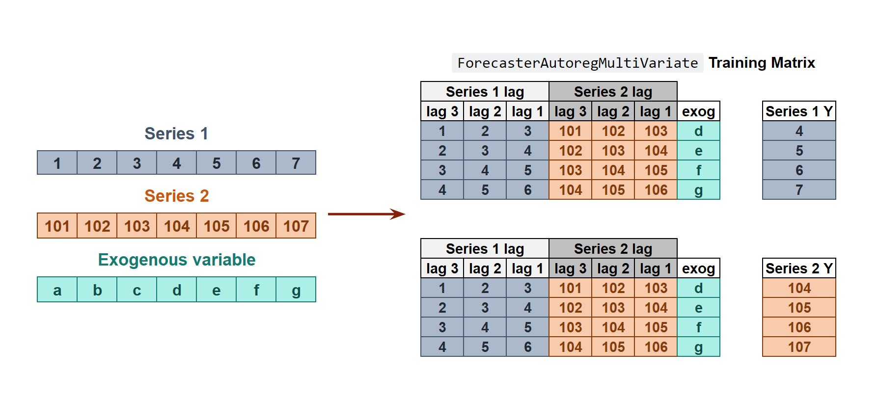
Internal Forecaster time series transformation to train a forecaster with multiple dependent time series.

Since a separate training matrix is created for each series in the dataset, it is necessary to define the target level on which forecasting will be performed. To predict the next n steps, one model is trained for each forecast horizon step. In the example shown, the selected level is Series 1.

This approach corresponds to a direct multi-step forecasting strategy, where each step is predicted independently using a separate model.

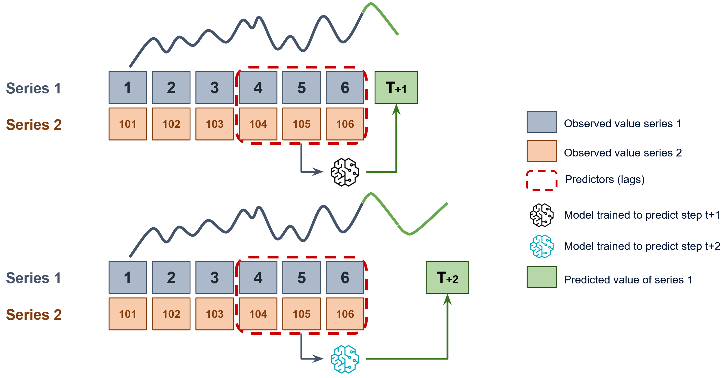
Diagram of direct forecasting with multiple dependent time series.

Using the ForecasterDirectMultiVariate class, it is possible to easily build machine learning models for multivariate forecasting.

💡 Tip

Why can only one series be predicted?

Direct forecasting strategies face a scalability challenge.

To predict multiple time series and multiple time steps, you would need a separate model for each series and each future time step. For example, with 1,000 series and a forecast horizon of 24, this would require training 24,000 individual models, a computationally impractical approach.

That’s why the ForecasterDirectMultiVariate can learn from multiple series, but can only predict one series at a time.

Looking for true multivariate with multiple series?

Try our ForecasterRnn class, which can handle multivariate forecasting with multiple series and multiple steps in a single deep learning model.

✎ Note

Skforecast offers additional approaches to create Global Forecasting Models:

• Global Forecasting Models: Independent multi-series forecasting
• Global Forecasting Models: Time series with different lengths and different exogenous variables
• Global Forecasting Models: Forecasting with Deep Learning

To learn more about global forecasting models visit our examples:

• Global Forecasting Models: Multi-series forecasting with Python and skforecast
• Scalable Forecasting: Modeling thousand time series with a single global model
• Global Forecasting Models: Comparative Analysis of Single and Multi-Series Forecasting Modeling
• Forecasting with Deep Learning

Libraries and data¶

In [1]:

# Libraries
# ==============================================================================
import numpy as np
import matplotlib.pyplot as plt
from sklearn.preprocessing import StandardScaler
from lightgbm import LGBMRegressor
from sklearn.metrics import mean_absolute_error
from skforecast.datasets import fetch_dataset
from skforecast.preprocessing import RollingFeatures
from skforecast.direct import ForecasterDirectMultiVariate
from skforecast.model_selection import (
    OneStepAheadFold,
    TimeSeriesFold,
    backtesting_forecaster_multiseries,
    grid_search_forecaster_multiseries,
    random_search_forecaster_multiseries,
    bayesian_search_forecaster_multiseries
)
from skforecast.plot import set_dark_theme

# Libraries # ============================================================================== import numpy as np import matplotlib.pyplot as plt from sklearn.preprocessing import StandardScaler from lightgbm import LGBMRegressor from sklearn.metrics import mean_absolute_error from skforecast.datasets import fetch_dataset from skforecast.preprocessing import RollingFeatures from skforecast.direct import ForecasterDirectMultiVariate from skforecast.model_selection import ( OneStepAheadFold, TimeSeriesFold, backtesting_forecaster_multiseries, grid_search_forecaster_multiseries, random_search_forecaster_multiseries, bayesian_search_forecaster_multiseries ) from skforecast.plot import set_dark_theme

In [2]:

# Data download
# ==============================================================================
data = fetch_dataset(name="air_quality_valencia_no_missing")

# Data download # ============================================================================== data = fetch_dataset(name="air_quality_valencia_no_missing")

air_quality_valencia_no_missing
-------------------------------
Hourly measures of several air chemical pollutant at Valencia city (Avd.
Francia) from 2019-01-01 to 20213-12-31. Including the following variables:
pm2.5 (µg/m³), CO (mg/m³), NO (µg/m³), NO2 (µg/m³), PM10 (µg/m³), NOx (µg/m³),
O3 (µg/m³), Veloc. (m/s), Direc. (degrees), SO2 (µg/m³). Missing values have
been imputed using linear interpolation.
Red de Vigilancia y Control de la Contaminación Atmosférica, 46250047-València -
Av. França, https://mediambient.gva.es/es/web/calidad-ambiental/datos-
historicos.
Shape of the dataset: (43824, 10)

In [3]:

# Aggregate at daily frequency to reduce dimensions
# ==============================================================================
data = data.resample('D').mean()
print("Shape: ", data.shape)
data.head()

# Aggregate at daily frequency to reduce dimensions # ============================================================================== data = data.resample('D').mean() print("Shape: ", data.shape) data.head()

Shape:  (1826, 10)

Out[3]:

	so2	co	no	no2	pm10	nox	o3	veloc.	direc.	pm2.5
datetime
2019-01-01	6.000000	0.141667	17.375000	37.250000	21.458333	63.458333	20.291667	0.416667	207.416667	17.208333
2019-01-02	6.041667	0.170833	23.458333	49.333333	26.416667	85.041667	11.708333	0.579167	225.375000	17.375000
2019-01-03	5.916667	0.216667	41.291667	53.250000	36.166667	116.333333	9.833333	0.500000	211.833333	21.625000
2019-01-04	5.458333	0.204167	21.208333	45.750000	32.208333	77.958333	15.166667	0.675000	199.583333	22.166667
2019-01-05	4.541667	0.191667	10.291667	36.375000	32.875000	51.833333	21.083333	0.875000	254.208333	24.916667

In [4]:

# Split data into train-val-test
# ==============================================================================
end_train = '2023-05-31 23:59:59'
data_train = data.loc[:end_train, :].copy()
data_test  = data.loc[end_train:, :].copy()

print(
    f"Train dates : {data_train.index.min()} --- {data_train.index.max()}  "
    f"(n={len(data_train)})"
)
print(
    f"Test dates  : {data_test.index.min()} --- {data_test.index.max()}  "
    f"(n={len(data_test)})"
)

# Split data into train-val-test # ============================================================================== end_train = '2023-05-31 23:59:59' data_train = data.loc[:end_train, :].copy() data_test = data.loc[end_train:, :].copy() print( f"Train dates : {data_train.index.min()} --- {data_train.index.max()} " f"(n={len(data_train)})" ) print( f"Test dates : {data_test.index.min()} --- {data_test.index.max()} " f"(n={len(data_test)})" )

Train dates : 2019-01-01 00:00:00 --- 2023-05-31 00:00:00  (n=1612)
Test dates  : 2023-06-01 00:00:00 --- 2023-12-31 00:00:00  (n=214)

In [5]:

# Plot time series
# ==============================================================================
set_dark_theme()
fig, axes = plt.subplots(nrows=3, ncols=1, figsize=(8, 5), sharex=True)
for i, col in enumerate(data.columns[:3]):
    data_train[col].plot(ax=axes[i], label='train')
    data_test[col].plot(ax=axes[i], label='test')
    axes[i].set_ylabel('Concentration(ug/m^3)', fontsize=8)
    axes[i].set_title(col)
    axes[i].legend(loc='upper right')

fig.tight_layout()
plt.show();

# Plot time series # ============================================================================== set_dark_theme() fig, axes = plt.subplots(nrows=3, ncols=1, figsize=(8, 5), sharex=True) for i, col in enumerate(data.columns[:3]): data_train[col].plot(ax=axes[i], label='train') data_test[col].plot(ax=axes[i], label='test') axes[i].set_ylabel('Concentration(ug/m^3)', fontsize=8) axes[i].set_title(col) axes[i].legend(loc='upper right') fig.tight_layout() plt.show();

Train and predict ForecasterDirectMultiVariate¶

When initializing the forecaster, the series (level) to be predicted and the maximum number of steps must be indicated since a different model will be created for each step.

✎ Note

ForecasterDirectMultiVariate includes the n_jobs argument, allowing multi-process parallelization to train regressors for all steps simultaneously, significantly reducing training time.

Its effectiveness depends on factors like the regressor type, the number of model fits to perform, and the volume of data. When n_jobs is set to 'auto', the level of parallelization is automatically determined using heuristic rules designed to select the most efficient configuration for each scenario.

For more information, see the guide Parallelization in skforecast.

In [6]:

# Create and fit forecaster MultiVariate
# ==============================================================================
forecaster = ForecasterDirectMultiVariate(
                 regressor          = LGBMRegressor(random_state=123, verbose=-1),
                 level              = 'co',
                 steps              = 7,
                 lags               = 7,
                 window_features    = RollingFeatures(stats=['mean'], window_sizes=[7]),
                 transformer_series = None,
                 transformer_exog   = None
             )

forecaster.fit(series=data_train)
forecaster

# Create and fit forecaster MultiVariate # ============================================================================== forecaster = ForecasterDirectMultiVariate( regressor = LGBMRegressor(random_state=123, verbose=-1), level = 'co', steps = 7, lags = 7, window_features = RollingFeatures(stats=['mean'], window_sizes=[7]), transformer_series = None, transformer_exog = None ) forecaster.fit(series=data_train) forecaster

Out[6]:

ForecasterDirectMultiVariate

General Information

• Regressor: LGBMRegressor
• Target series (level): co
• Lags: [1 2 3 4 5 6 7]
• Window features: ['roll_mean_7']
• Window size: 7
• Maximum steps to predict: 7
• Exogenous included: False
• Weight function included: False
• Differentiation order: None
• Creation date: 2025-08-06 13:39:31
• Last fit date: 2025-08-06 13:39:37
• Skforecast version: 0.17.0
• Python version: 3.12.11
• Forecaster id: None

Exogenous Variables

None

Data Transformations

• Transformer for series: None
• Transformer for exog: None

Training Information

• Target series (level): co
• Multivariate series: so2, co, no, no2, pm10, nox, o3, veloc., direc., pm2.5
• Training range: [Timestamp('2019-01-01 00:00:00'), Timestamp('2023-05-31 00:00:00')]
• Training index type: DatetimeIndex
• Training index frequency: D

Regressor Parameters

{'boosting_type': 'gbdt', 'class_weight': None, 'colsample_bytree': 1.0, 'importance_type': 'split', 'learning_rate': 0.1, 'max_depth': -1, 'min_child_samples': 20, 'min_child_weight': 0.001, 'min_split_gain': 0.0, 'n_estimators': 100, 'n_jobs': None, 'num_leaves': 31, 'objective': None, 'random_state': 123, 'reg_alpha': 0.0, 'reg_lambda': 0.0, 'subsample': 1.0, 'subsample_for_bin': 200000, 'subsample_freq': 0, 'verbose': -1}

Fit Kwargs

{}

🛈 API Reference    🗎 User Guide

When predicting, the value of steps must be less than or equal to the value of steps defined when initializing the forecaster. Starts at 1.

• If int only steps within the range of 1 to int are predicted.

• If list of int. Only the steps contained in the list are predicted.

• If None as many steps are predicted as were defined at initialization.

In [7]:

# Predict with forecaster MultiVariate
# ==============================================================================
predictions = forecaster.predict(steps=None)  # All steps
predictions

# Predict with forecaster MultiVariate # ============================================================================== predictions = forecaster.predict(steps=None) # All steps predictions

Out[7]:

	level	pred
2023-06-01	co	0.100165
2023-06-02	co	0.108636
2023-06-03	co	0.113710
2023-06-04	co	0.103102
2023-06-05	co	0.105516
2023-06-06	co	0.114029
2023-06-07	co	0.110274

In [8]:

# Predict only a subset of steps
# ==============================================================================
predictions = forecaster.predict(steps=[1, 5])
predictions

# Predict only a subset of steps # ============================================================================== predictions = forecaster.predict(steps=[1, 5]) predictions

Out[8]:

	level	pred
2023-06-01	co	0.100165
2023-06-05	co	0.105516

In [9]:

# Predict intervals using in-sample residuals
# ==============================================================================
forecaster.set_in_sample_residuals(series=data_train)
predictions = forecaster.predict_interval(random_state=9871)
predictions

# Predict intervals using in-sample residuals # ============================================================================== forecaster.set_in_sample_residuals(series=data_train) predictions = forecaster.predict_interval(random_state=9871) predictions

Out[9]:

	level	pred	lower_bound	upper_bound
2023-06-01	co	0.100165	0.096533	0.103797
2023-06-02	co	0.108636	0.099615	0.117657
2023-06-03	co	0.113710	0.101929	0.125490
2023-06-04	co	0.103102	0.099967	0.106237
2023-06-05	co	0.105516	0.099785	0.111247
2023-06-06	co	0.114029	0.102248	0.125810
2023-06-07	co	0.110274	0.098493	0.122054

To learn more about probabilistic forecasting features available in skforecast, see the probabilistic forecasting user guides.

Backtesting MultiVariate¶

See the backtesting user guide to learn more about backtesting.

In [10]:

# Backtesting MultiVariate
# ==============================================================================
cv = TimeSeriesFold(
         steps                 = 7,
         initial_train_size    = len(data_train),
         refit                 = False,
         allow_incomplete_fold = True
     )

metrics_levels, backtest_preds = backtesting_forecaster_multiseries(
                                     forecaster = forecaster,
                                     series     = data,
                                     cv         = cv,
                                     metric     = 'mean_absolute_error'
                                 )
display(metrics_levels)
backtest_preds.head(4)

# Backtesting MultiVariate # ============================================================================== cv = TimeSeriesFold( steps = 7, initial_train_size = len(data_train), refit = False, allow_incomplete_fold = True ) metrics_levels, backtest_preds = backtesting_forecaster_multiseries( forecaster = forecaster, series = data, cv = cv, metric = 'mean_absolute_error' ) display(metrics_levels) backtest_preds.head(4)

  0%|          | 0/31 [00:00<?, ?it/s]

	levels	mean_absolute_error
0	co	0.016993

Out[10]:

	level	pred
2023-06-01	co	0.100165
2023-06-02	co	0.108636
2023-06-03	co	0.113710
2023-06-04	co	0.103102

Hyperparameter tuning and lags selection MultiVariate¶

Hyperparameter tuning consists of systematically evaluating combinations of hyperparameters (including lags) to find the configuration that yields the best predictive performance. The skforecast library supports several tuning strategies: grid search, random search, and Bayesian search. These strategies can be used with either backtesting or one-step-ahead validation to determine the optimal parameter set for a given forecasting task.

The functions grid_search_forecaster_multiseries, random_search_forecaster_multiseries and bayesian_search_forecaster_multiseries from the model_selection module allow for lags and hyperparameter optimization.

The following example shows how to use random_search_forecaster_multiseries to find the best lags and model hyperparameters.

In [11]:

# Create and forecaster MultiVariate
# ==============================================================================
forecaster = ForecasterDirectMultiVariate(
                 regressor       = LGBMRegressor(random_state=123, verbose=-1),
                 level           = 'co',
                 steps           = 7,
                 lags            = 7,
                 window_features = RollingFeatures(stats=['mean'], window_sizes=[7])
             )

# Create and forecaster MultiVariate # ============================================================================== forecaster = ForecasterDirectMultiVariate( regressor = LGBMRegressor(random_state=123, verbose=-1), level = 'co', steps = 7, lags = 7, window_features = RollingFeatures(stats=['mean'], window_sizes=[7]) )

In [12]:

# Random search MultiVariate
# ==============================================================================
lags_grid = [7, 14]
param_distributions = {
    'n_estimators': np.arange(start=10, stop=20, step=1, dtype=int),
    'max_depth': np.arange(start=3, stop=6, step=1, dtype=int)
}

cv = TimeSeriesFold(
         steps              = 7,
         initial_train_size = len(data_train),
         refit              = False,
     )

results = random_search_forecaster_multiseries(
              forecaster          = forecaster,
              series              = data,
              lags_grid           = lags_grid,
              param_distributions = param_distributions,
              cv                  = cv,
              metric              = 'mean_absolute_error',
              n_iter              = 5,
          )

results

# Random search MultiVariate # ============================================================================== lags_grid = [7, 14] param_distributions = { 'n_estimators': np.arange(start=10, stop=20, step=1, dtype=int), 'max_depth': np.arange(start=3, stop=6, step=1, dtype=int) } cv = TimeSeriesFold( steps = 7, initial_train_size = len(data_train), refit = False, ) results = random_search_forecaster_multiseries( forecaster = forecaster, series = data, lags_grid = lags_grid, param_distributions = param_distributions, cv = cv, metric = 'mean_absolute_error', n_iter = 5, ) results

lags grid:   0%|          | 0/2 [00:00<?, ?it/s]

params grid:   0%|          | 0/5 [00:00<?, ?it/s]

`Forecaster` refitted using the best-found lags and parameters, and the whole data set: 
  Lags: [ 1  2  3  4  5  6  7  8  9 10 11 12 13 14] 
  Parameters: {'n_estimators': np.int64(19), 'max_depth': np.int64(5)}
  Backtesting metric: 0.016567112132881933
  Levels: ['co']

Out[12]:

	levels	lags	lags_label	params	mean_absolute_error	n_estimators	max_depth
0	[co]	[1, 2, 3, 4, 5, 6, 7, 8, 9, 10, 11, 12, 13, 14]	[1, 2, 3, 4, 5, 6, 7, 8, 9, 10, 11, 12, 13, 14]	{'n_estimators': 19, 'max_depth': 5}	0.016567	19	5
1	[co]	[1, 2, 3, 4, 5, 6, 7, 8, 9, 10, 11, 12, 13, 14]	[1, 2, 3, 4, 5, 6, 7, 8, 9, 10, 11, 12, 13, 14]	{'n_estimators': 16, 'max_depth': 5}	0.017329	16	5
2	[co]	[1, 2, 3, 4, 5, 6, 7]	[1, 2, 3, 4, 5, 6, 7]	{'n_estimators': 18, 'max_depth': 3}	0.017705	18	3
3	[co]	[1, 2, 3, 4, 5, 6, 7]	[1, 2, 3, 4, 5, 6, 7]	{'n_estimators': 19, 'max_depth': 5}	0.017724	19	5
4	[co]	[1, 2, 3, 4, 5, 6, 7, 8, 9, 10, 11, 12, 13, 14]	[1, 2, 3, 4, 5, 6, 7, 8, 9, 10, 11, 12, 13, 14]	{'n_estimators': 18, 'max_depth': 3}	0.017854	18	3
5	[co]	[1, 2, 3, 4, 5, 6, 7]	[1, 2, 3, 4, 5, 6, 7]	{'n_estimators': 17, 'max_depth': 3}	0.017885	17	3
6	[co]	[1, 2, 3, 4, 5, 6, 7]	[1, 2, 3, 4, 5, 6, 7]	{'n_estimators': 16, 'max_depth': 5}	0.017923	16	5
7	[co]	[1, 2, 3, 4, 5, 6, 7, 8, 9, 10, 11, 12, 13, 14]	[1, 2, 3, 4, 5, 6, 7, 8, 9, 10, 11, 12, 13, 14]	{'n_estimators': 15, 'max_depth': 3}	0.018076	15	3
8	[co]	[1, 2, 3, 4, 5, 6, 7, 8, 9, 10, 11, 12, 13, 14]	[1, 2, 3, 4, 5, 6, 7, 8, 9, 10, 11, 12, 13, 14]	{'n_estimators': 17, 'max_depth': 3}	0.018101	17	3
9	[co]	[1, 2, 3, 4, 5, 6, 7]	[1, 2, 3, 4, 5, 6, 7]	{'n_estimators': 15, 'max_depth': 3}	0.018235	15	3

It is also possible to perform a bayesian optimization with Optuna using the bayesian_search_forecaster_multiseries function. For more information about this type of optimization, visit the user guide.

In [26]:

# Bayesian search hyperparameters and lags with Optuna
# ==============================================================================
forecaster = ForecasterDirectMultiVariate(
                 regressor       = LGBMRegressor(random_state=123, verbose=-1),
                 level           = 'co',
                 steps           = 7,
                 lags            = 7,
                 window_features = RollingFeatures(stats=['mean'], window_sizes=[7])
             )

# Search space
def search_space(trial):
    search_space  = {
        'lags'            : trial.suggest_categorical('lags', [7, 14]),
        'n_estimators'    : trial.suggest_int('n_estimators', 10, 20),
        'min_samples_leaf': trial.suggest_int('min_samples_leaf', 1., 10),
        'max_features'    : trial.suggest_categorical('max_features', ['log2', 'sqrt'])
    }

    return search_space

cv = OneStepAheadFold(initial_train_size = '2023-05-31 23:59:59')

results, best_trial = bayesian_search_forecaster_multiseries(
                          forecaster            = forecaster,
                          series                = data,
                          search_space          = search_space,
                          cv                    = cv,
                          metric                = 'mean_absolute_error',
                          n_trials              = 5,
                          kwargs_create_study   = {},
                          kwargs_study_optimize = {}
                      )

results.head(4)

# Bayesian search hyperparameters and lags with Optuna # ============================================================================== forecaster = ForecasterDirectMultiVariate( regressor = LGBMRegressor(random_state=123, verbose=-1), level = 'co', steps = 7, lags = 7, window_features = RollingFeatures(stats=['mean'], window_sizes=[7]) ) # Search space def search_space(trial): search_space = { 'lags' : trial.suggest_categorical('lags', [7, 14]), 'n_estimators' : trial.suggest_int('n_estimators', 10, 20), 'min_samples_leaf': trial.suggest_int('min_samples_leaf', 1., 10), 'max_features' : trial.suggest_categorical('max_features', ['log2', 'sqrt']) } return search_space cv = OneStepAheadFold(initial_train_size = '2023-05-31 23:59:59') results, best_trial = bayesian_search_forecaster_multiseries( forecaster = forecaster, series = data, search_space = search_space, cv = cv, metric = 'mean_absolute_error', n_trials = 5, kwargs_create_study = {}, kwargs_study_optimize = {} ) results.head(4)

  0%|          | 0/5 [00:00<?, ?it/s]

`Forecaster` refitted using the best-found lags and parameters, and the whole data set: 
  Lags: [ 1  2  3  4  5  6  7  8  9 10 11 12 13 14] 
  Parameters: {'n_estimators': 16, 'min_samples_leaf': 9, 'max_features': 'log2'}
  Backtesting metric: 0.010437198123137972
  Levels: ['co']

c:\Users\jaesc2\Miniconda3\envs\skforecast_py12\Lib\site-packages\jupyter_client\session.py:203: DeprecationWarning: datetime.datetime.utcnow() is deprecated and scheduled for removal in a future version. Use timezone-aware objects to represent datetimes in UTC: datetime.datetime.now(datetime.UTC).
  return datetime.utcnow().replace(tzinfo=utc)
c:\Users\jaesc2\Miniconda3\envs\skforecast_py12\Lib\site-packages\jupyter_client\session.py:203: DeprecationWarning: datetime.datetime.utcnow() is deprecated and scheduled for removal in a future version. Use timezone-aware objects to represent datetimes in UTC: datetime.datetime.now(datetime.UTC).
  return datetime.utcnow().replace(tzinfo=utc)

Out[26]:

	levels	lags	params	mean_absolute_error	n_estimators	min_samples_leaf	max_features
0	[co]	[1, 2, 3, 4, 5, 6, 7, 8, 9, 10, 11, 12, 13, 14]	{'n_estimators': 16, 'min_samples_leaf': 9, 'm...	0.010437	16	9	log2
1	[co]	[1, 2, 3, 4, 5, 6, 7]	{'n_estimators': 15, 'min_samples_leaf': 4, 'm...	0.010891	15	4	sqrt
2	[co]	[1, 2, 3, 4, 5, 6, 7]	{'n_estimators': 14, 'min_samples_leaf': 8, 'm...	0.011436	14	8	log2
3	[co]	[1, 2, 3, 4, 5, 6, 7]	{'n_estimators': 12, 'min_samples_leaf': 6, 'm...	0.012376	12	6	log2

The best_trial return contains the details of the trial that achieved the best result during optimization. For more information, refer to the Study class.

In [15]:

# Optuna best trial in the study
# ==============================================================================
best_trial

# Optuna best trial in the study # ============================================================================== best_trial

Out[15]:

FrozenTrial(number=3, state=1, values=[0.010437198123137972], datetime_start=datetime.datetime(2025, 8, 6, 13, 39, 52, 376342), datetime_complete=datetime.datetime(2025, 8, 6, 13, 39, 52, 540519), params={'lags': 14, 'n_estimators': 16, 'min_samples_leaf': 9, 'max_features': 'log2'}, user_attrs={}, system_attrs={}, intermediate_values={}, distributions={'lags': CategoricalDistribution(choices=(7, 14)), 'n_estimators': IntDistribution(high=20, log=False, low=10, step=1), 'min_samples_leaf': IntDistribution(high=10, log=False, low=1, step=1), 'max_features': CategoricalDistribution(choices=('log2', 'sqrt'))}, trial_id=3, value=None)

Different lags for each time series¶

Passing a dict to the lags argument allows specifying different lags for each time series. The dictionary keys must correspond to the names of the series used during training, and the values define the lags to be applied to each one individually.

In [28]:

# Create and fit forecaster MultiVariate Custom lags
# ==============================================================================
lags_dict = {
    'so2': [7, 14], 'co': 7, 'no': [7, 14], 'no2': [7, 14],
    'pm10': [7, 14], 'nox': [7, 14], 'o3': [7, 14], 'veloc.': 3,
    'direc.': 3, 'pm2.5': [7, 14]
}
forecaster = ForecasterDirectMultiVariate(
                 regressor = LGBMRegressor(random_state=123, verbose=-1),
                 level     = 'co',
                 steps     = 7,
                 lags      = lags_dict,
             )

forecaster.fit(series=data_train)

# Predict
# ==============================================================================
predictions = forecaster.predict(steps=7)
predictions

# Create and fit forecaster MultiVariate Custom lags # ============================================================================== lags_dict = { 'so2': [7, 14], 'co': 7, 'no': [7, 14], 'no2': [7, 14], 'pm10': [7, 14], 'nox': [7, 14], 'o3': [7, 14], 'veloc.': 3, 'direc.': 3, 'pm2.5': [7, 14] } forecaster = ForecasterDirectMultiVariate( regressor = LGBMRegressor(random_state=123, verbose=-1), level = 'co', steps = 7, lags = lags_dict, ) forecaster.fit(series=data_train) # Predict # ============================================================================== predictions = forecaster.predict(steps=7) predictions

Out[28]:

	level	pred
2023-06-01	co	0.098798
2023-06-02	co	0.107185
2023-06-03	co	0.112225
2023-06-04	co	0.107208
2023-06-05	co	0.098643
2023-06-06	co	0.100375
2023-06-07	co	0.099513

If None is assigned to any key in the lags dictionary, that series will be excluded from the creation of the X training matrix.

In the following example, no lags are generated for the 'co' series. However, since 'co' is the specified target level, its values are still used to construct the y training matrix.

In [29]:

# Create and fit forecaster MultiVariate Custom lags with None
# ==============================================================================
lags_dict = {
    'so2': [7, 14], 'co': None, 'no': [7, 14], 'no2': [7, 14],
    'pm10': [7, 14], 'nox': [7, 14], 'o3': [7, 14], 'veloc.': 3,
    'direc.': 3, 'pm2.5': [7, 14]
}
forecaster = ForecasterDirectMultiVariate(
                 regressor = LGBMRegressor(random_state=123, verbose=-1),
                 level     = 'co',
                 lags      = lags_dict,
                 steps     = 7,
             )

forecaster.fit(series=data_train)

# Predict
# ==============================================================================
predictions = forecaster.predict(steps=7)
predictions

# Create and fit forecaster MultiVariate Custom lags with None # ============================================================================== lags_dict = { 'so2': [7, 14], 'co': None, 'no': [7, 14], 'no2': [7, 14], 'pm10': [7, 14], 'nox': [7, 14], 'o3': [7, 14], 'veloc.': 3, 'direc.': 3, 'pm2.5': [7, 14] } forecaster = ForecasterDirectMultiVariate( regressor = LGBMRegressor(random_state=123, verbose=-1), level = 'co', lags = lags_dict, steps = 7, ) forecaster.fit(series=data_train) # Predict # ============================================================================== predictions = forecaster.predict(steps=7) predictions

Out[29]:

	level	pred
2023-06-01	co	0.107966
2023-06-02	co	0.118692
2023-06-03	co	0.125480
2023-06-04	co	0.132908
2023-06-05	co	0.118237
2023-06-06	co	0.121638
2023-06-07	co	0.120753

It is possible to use the create_train_X_y method to generate the matrices that the forecaster is using to train the model. This approach enables gaining insight into the specific lags that have been created.

In [30]:

# Extract training matrix
# ==============================================================================
X_train, y_train = forecaster.create_train_X_y(series=data_train)

# X and y to train model for step 1
X_train_step_1, y_train_step_1 = forecaster.filter_train_X_y_for_step(
                                     step    = 1,
                                     X_train = X_train,
                                     y_train = y_train,
                                 )

X_train_step_1.head(4)

# Extract training matrix # ============================================================================== X_train, y_train = forecaster.create_train_X_y(series=data_train) # X and y to train model for step 1 X_train_step_1, y_train_step_1 = forecaster.filter_train_X_y_for_step( step = 1, X_train = X_train, y_train = y_train, ) X_train_step_1.head(4)

Out[30]:

	so2_lag_7	so2_lag_14	no_lag_7	no_lag_14	no2_lag_7	no2_lag_14	pm10_lag_7	pm10_lag_14	nox_lag_7	nox_lag_14	o3_lag_7	o3_lag_14	veloc._lag_1	veloc._lag_2	veloc._lag_3	direc._lag_1	direc._lag_2	direc._lag_3	pm2.5_lag_7	pm2.5_lag_14
datetime
2019-01-15	1.061795	2.362414	3.462136	2.232968	2.971237	2.098158	1.175259	0.229121	3.419881	2.298657	-1.871669	-1.800847	-0.726869	-0.979544	-0.792953	0.673274	1.019948	1.581166	2.104497	1.084751
2019-01-16	1.805006	2.408865	6.247303	3.270300	2.622404	3.254290	1.156585	0.599485	4.605306	3.486375	-1.754371	-2.256761	-1.150585	-0.726869	-0.979544	0.171311	0.673274	1.019948	1.782163	1.108193
2019-01-17	-0.982034	2.269513	0.826174	6.311248	2.596491	3.629037	-0.119456	1.327762	1.927209	5.208336	-0.331300	-2.356354	-0.944558	-1.150585	-0.726869	0.511174	0.171311	0.673274	-0.374541	1.705975
2019-01-18	1.479852	1.758556	8.194077	2.886629	4.617729	2.911437	1.221944	1.032094	6.726230	3.096583	-1.433461	-2.073068	-1.115600	-0.944558	-1.150585	1.436094	0.511174	0.171311	0.815163	1.782163

In [31]:

# Extract training matrix
# ==============================================================================
y_train_step_1.head(4)

# Extract training matrix # ============================================================================== y_train_step_1.head(4)

Out[31]:

datetime
2019-01-15    3.149604
2019-01-16    1.554001
2019-01-17   -0.323179
2019-01-18   -0.417038
Freq: D, Name: co_step_1, dtype: float64

Exogenous variables in MultiVariate¶

Exogenous variables are predictors that are independent of the model being used for forecasting, and their future values must be known in order to include them in the prediction process.

In the ForecasterDirectMultiVariate, as in the other forecasters, exogenous variables can be easily included as predictors using the exog argument.

To learn more about exogenous variables in skforecast visit the exogenous variables user guide.

Scikit-learn transformers in MultiVariate¶

By default, the ForecasterDirectMultiVariate class uses the scikit-learn StandardScaler transformer to scale the data. This transformer is applied to all series. However, it is possible to use different transformers for each series or not to apply any transformation at all:

• If transformer_series is a transformer the same transformation will be applied to all series.

• If transformer_series is a dict a different transformation can be set for each series. Series not present in the dict will not have any transformation applied to them (check warning message).

Learn more about using scikit-learn transformers with skforecast.

In [32]:

# Transformers in MultiVariate
# ==============================================================================
forecaster = ForecasterDirectMultiVariate(
                 regressor          = LGBMRegressor(random_state=123, verbose=-1),
                 level              = 'co',
                 lags               = 7,
                 steps              = 7,
                 transformer_series = {'co': StandardScaler(), 'no2': StandardScaler()}
             )

forecaster.fit(series=data_train)
forecaster

# Transformers in MultiVariate # ============================================================================== forecaster = ForecasterDirectMultiVariate( regressor = LGBMRegressor(random_state=123, verbose=-1), level = 'co', lags = 7, steps = 7, transformer_series = {'co': StandardScaler(), 'no2': StandardScaler()} ) forecaster.fit(series=data_train) forecaster

╭─────────────────────────────── IgnoredArgumentWarning ───────────────────────────────╮
│ {'pm2.5', 'pm10', 'no', 'so2', 'veloc.', 'o3', 'direc.', 'nox'} not present in       │
│ `transformer_series`. No transformation is applied to these series.                  │
│                                                                                      │
│ Category : IgnoredArgumentWarning                                                    │
│ Location :                                                                           │
│ c:\Users\jaesc2\Miniconda3\envs\skforecast_py12\Lib\site-packages\skforecast\utils\u │
│ tils.py:372                                                                          │
│ Suppress : warnings.simplefilter('ignore', category=IgnoredArgumentWarning)          │
╰──────────────────────────────────────────────────────────────────────────────────────╯

Out[32]:

ForecasterDirectMultiVariate

General Information

• Regressor: LGBMRegressor
• Target series (level): co
• Lags: [1 2 3 4 5 6 7]
• Window features: None
• Window size: 7
• Maximum steps to predict: 7
• Exogenous included: False
• Weight function included: False
• Differentiation order: None
• Creation date: 2025-08-06 13:40:51
• Last fit date: 2025-08-06 13:40:52
• Skforecast version: 0.17.0
• Python version: 3.12.11
• Forecaster id: None

Exogenous Variables

None

Data Transformations

• Transformer for series: 'co': StandardScaler(), 'no2': StandardScaler()
• Transformer for exog: None

Training Information

• Target series (level): co
• Multivariate series: so2, co, no, no2, pm10, nox, o3, veloc., direc., pm2.5
• Training range: [Timestamp('2019-01-01 00:00:00'), Timestamp('2023-05-31 00:00:00')]
• Training index type: DatetimeIndex
• Training index frequency: D

Regressor Parameters

{'boosting_type': 'gbdt', 'class_weight': None, 'colsample_bytree': 1.0, 'importance_type': 'split', 'learning_rate': 0.1, 'max_depth': -1, 'min_child_samples': 20, 'min_child_weight': 0.001, 'min_split_gain': 0.0, 'n_estimators': 100, 'n_jobs': None, 'num_leaves': 31, 'objective': None, 'random_state': 123, 'reg_alpha': 0.0, 'reg_lambda': 0.0, 'subsample': 1.0, 'subsample_for_bin': 200000, 'subsample_freq': 0, 'verbose': -1}

Fit Kwargs

{}

🛈 API Reference    🗎 User Guide

Weights in MultiVariate¶

The weights are used to control the influence that each observation has on the training of the model.

Learn more about weighted time series forecasting with skforecast.

In [33]:

# Weights in MultiVariate
# ==============================================================================
def custom_weights(index):
    """
    Return 0 if index is between '2013-01-01' and '2013-01-31', 1 otherwise.
    """
    weights = np.where(
                  (index >= '2013-01-01') & (index <= '2013-01-31'),
                   0,
                   1
              )
    
    return weights


forecaster = ForecasterDirectMultiVariate(
                 regressor          = LGBMRegressor(random_state=123, verbose=-1),
                 level              = 'co',
                 lags               = 7,
                 steps              = 7,
                 transformer_series = StandardScaler(),
                 weight_func        = custom_weights
             )

forecaster.fit(series=data_train)
forecaster.predict(steps=7).head(3)

# Weights in MultiVariate # ============================================================================== def custom_weights(index): """ Return 0 if index is between '2013-01-01' and '2013-01-31', 1 otherwise. """ weights = np.where( (index >= '2013-01-01') & (index <= '2013-01-31'), 0, 1 ) return weights forecaster = ForecasterDirectMultiVariate( regressor = LGBMRegressor(random_state=123, verbose=-1), level = 'co', lags = 7, steps = 7, transformer_series = StandardScaler(), weight_func = custom_weights ) forecaster.fit(series=data_train) forecaster.predict(steps=7).head(3)

Out[33]:

	level	pred
2023-06-01	co	0.106243
2023-06-02	co	0.103617
2023-06-03	co	0.102537

⚠ Warning

The weight_func argument will be ignored if the regressor does not accept sample_weight in its fit method.

The source code of the weight_func added to the forecaster is stored in the argument source_code_weight_func.

In [34]:

# Source code weight function
# ==============================================================================
print(forecaster.source_code_weight_func)

# Source code weight function # ============================================================================== print(forecaster.source_code_weight_func)

def custom_weights(index):
    """
    Return 0 if index is between '2013-01-01' and '2013-01-31', 1 otherwise.
    """
    weights = np.where(
                  (index >= '2013-01-01') & (index <= '2013-01-31'),
                   0,
                   1
              )

    return weights

Compare multiple metrics¶

The functions backtesting_forecaster_multiseries, grid_search_forecaster_multiseries, random_search_forecaster_multiseries, and bayesian_search_forecaster_multiseries support the evaluation of multiple metrics by passing a list of metric functions. This list can include both built-in metrics (e.g. mean_squared_error, mean_absolute_error) and custom-defined ones.

When multiple metrics are provided, the first metric in the list is used to select the best model.

💡 Tip

More information about time series forecasting metrics can be found in the Metrics guide.

In [35]:

# Grid search MultiVariate with multiple metrics
# ==============================================================================
forecaster = ForecasterDirectMultiVariate(
                 regressor = LGBMRegressor(random_state=123, verbose=-1),
                 level     = 'co',
                 lags      = 7,
                 steps     = 7
             )    

def custom_metric(y_true, y_pred):
    """
    Calculate the mean absolute error using only the predicted values of the last
    3 months of the year.
    """
    mask = y_true.index.month.isin([10, 11, 12])
    metric = mean_absolute_error(y_true[mask], y_pred[mask])
    
    return metric

cv = TimeSeriesFold(
         steps              = 7,
         initial_train_size = len(data_train),
         refit              = False,
     )

lags_grid = [7, 14]
param_grid = {'alpha': [0.01, 0.1, 1]}

results = grid_search_forecaster_multiseries(
              forecaster = forecaster,
              series     = data,
              lags_grid  = lags_grid,
              param_grid = param_grid,
              cv         = cv,
              metric     = [mean_absolute_error, custom_metric, 'mean_squared_error']
          )

results

# Grid search MultiVariate with multiple metrics # ============================================================================== forecaster = ForecasterDirectMultiVariate( regressor = LGBMRegressor(random_state=123, verbose=-1), level = 'co', lags = 7, steps = 7 ) def custom_metric(y_true, y_pred): """ Calculate the mean absolute error using only the predicted values of the last 3 months of the year. """ mask = y_true.index.month.isin([10, 11, 12]) metric = mean_absolute_error(y_true[mask], y_pred[mask]) return metric cv = TimeSeriesFold( steps = 7, initial_train_size = len(data_train), refit = False, ) lags_grid = [7, 14] param_grid = {'alpha': [0.01, 0.1, 1]} results = grid_search_forecaster_multiseries( forecaster = forecaster, series = data, lags_grid = lags_grid, param_grid = param_grid, cv = cv, metric = [mean_absolute_error, custom_metric, 'mean_squared_error'] ) results

lags grid:   0%|          | 0/2 [00:00<?, ?it/s]

params grid:   0%|          | 0/3 [00:00<?, ?it/s]

`Forecaster` refitted using the best-found lags and parameters, and the whole data set: 
  Lags: [ 1  2  3  4  5  6  7  8  9 10 11 12 13 14] 
  Parameters: {'alpha': 0.01}
  Backtesting metric: 0.014486558378954958
  Levels: ['co']

Out[35]:

	levels	lags	lags_label	params	mean_absolute_error	custom_metric	mean_squared_error	alpha
0	[co]	[1, 2, 3, 4, 5, 6, 7, 8, 9, 10, 11, 12, 13, 14]	[1, 2, 3, 4, 5, 6, 7, 8, 9, 10, 11, 12, 13, 14]	{'alpha': 0.01}	0.014487	0.021981	0.000439	0.01
1	[co]	[1, 2, 3, 4, 5, 6, 7, 8, 9, 10, 11, 12, 13, 14]	[1, 2, 3, 4, 5, 6, 7, 8, 9, 10, 11, 12, 13, 14]	{'alpha': 0.1}	0.014487	0.021981	0.000439	0.10
2	[co]	[1, 2, 3, 4, 5, 6, 7, 8, 9, 10, 11, 12, 13, 14]	[1, 2, 3, 4, 5, 6, 7, 8, 9, 10, 11, 12, 13, 14]	{'alpha': 1}	0.014487	0.021981	0.000439	1.00
3	[co]	[1, 2, 3, 4, 5, 6, 7]	[1, 2, 3, 4, 5, 6, 7]	{'alpha': 0.01}	0.014773	0.022789	0.000511	0.01
4	[co]	[1, 2, 3, 4, 5, 6, 7]	[1, 2, 3, 4, 5, 6, 7]	{'alpha': 1}	0.014773	0.022789	0.000511	1.00
5	[co]	[1, 2, 3, 4, 5, 6, 7]	[1, 2, 3, 4, 5, 6, 7]	{'alpha': 0.1}	0.014773	0.022789	0.000511	0.10

Feature importances¶

Since ForecasterDirectMultiVariate fits one model per step, it is necessary to specify from which model retrieves its feature importances.

In [36]:

# Feature importances for step 1
# ==============================================================================
forecaster.get_feature_importances(step=1)

# Feature importances for step 1 # ============================================================================== forecaster.get_feature_importances(step=1)

Out[36]:

	feature	importance
14	co_lag_1	146
31	no_lag_4	84
61	pm10_lag_6	64
1	so2_lag_2	52
0	so2_lag_1	50
...	...	...
52	no2_lag_11	8
131	pm2.5_lag_6	8
132	pm2.5_lag_7	7
82	nox_lag_13	5
54	no2_lag_13	3

140 rows × 2 columns

Training and prediction matrices¶

While the primary goal of building forecasting models is to predict future values, it is equally important to evaluate if the model is effectively learning from the training data. Analyzing predictions on the training data or exploring the prediction matrices is crucial for assessing model performance and understanding areas for optimization. This process can help identify issues like overfitting or underfitting, as well as provide deeper insights into the model’s decision-making process. Check the How to Extract Training and Prediction Matrices user guide for more information.