Probabilistic Forecasting: Conformal Prediction¶

Conformal prediction is a framework for constructing prediction intervals that are guaranteed to contain the true value with a specified probability (coverage probability). It works by combining the predictions of a point-forecasting model with its past residuals—differences between previous predictions and actual values. These residuals help estimate the uncertainty in the forecast and determine the width of the prediction interval that is then added to the point forecast. Skforecast implements Split Conformal Prediction (SCP).

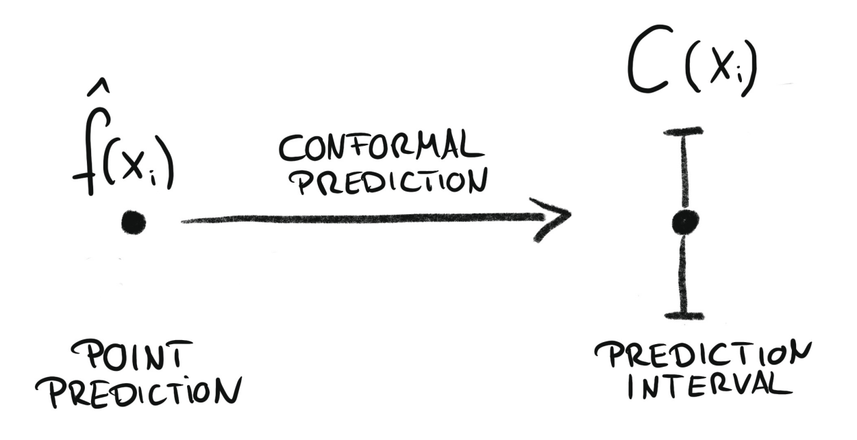
Conformal regression turns point predictions into prediction intervals. Source: Introduction To Conformal Prediction With Python: A Short Guide For Quantifying Uncertainty Of Machine Learning Models by Christoph Molnar https://leanpub.com/conformal-prediction

Conformal methods can also calibrate prediction intervals generated by other techniques, such as quantile regression or bootstrapped residuals. In this case, the conformal method adjusts the prediction intervals to ensure that they remain valid with respect to the coverage probability. Skforecast provides this functionality through the ConformalIntervalCalibrator transformer.

⚠ Warning

There are several well-established methods for conformal prediction, each with its own characteristics and assumptions. However, when applied to time series forecasting, their coverage guarantees are only valid for one-step-ahead predictions. For multi-step-ahead predictions, the coverage probability is not guaranteed. Skforecast implements Split Conformal Prediction (SCP) due to its simplicity and efficiency.

💡 Tip

For more examples on how to use probabilistic forecasting, check out the following articles:

• Probabilistic forecasting with machine learning
• Probabilistic forecasting: prediction intervals for multi-step time series forecasting
• Continuous Ranked Probability Score (CRPS) in probabilistic forecasting

Libraries and data¶

In [1]:

# Data processing
# ==============================================================================
import numpy as np
import pandas as pd
from skforecast.datasets import fetch_dataset

# Plots
# ==============================================================================
import matplotlib.pyplot as plt
from skforecast.plot import set_dark_theme, plot_residuals, plot_prediction_intervals

# Modelling and Forecasting
# ==============================================================================
from lightgbm import LGBMRegressor
from skforecast.recursive import ForecasterRecursive
from skforecast.preprocessing import RollingFeatures
from skforecast.model_selection import TimeSeriesFold, backtesting_forecaster
from skforecast.metrics import calculate_coverage

# Configuration
# ==============================================================================
import warnings
warnings.filterwarnings('once')

# Data processing # ============================================================================== import numpy as np import pandas as pd from skforecast.datasets import fetch_dataset # Plots # ============================================================================== import matplotlib.pyplot as plt from skforecast.plot import set_dark_theme, plot_residuals, plot_prediction_intervals # Modelling and Forecasting # ============================================================================== from lightgbm import LGBMRegressor from skforecast.recursive import ForecasterRecursive from skforecast.preprocessing import RollingFeatures from skforecast.model_selection import TimeSeriesFold, backtesting_forecaster from skforecast.metrics import calculate_coverage # Configuration # ============================================================================== import warnings warnings.filterwarnings('once')

In [2]:

# Data
# ==============================================================================
data = fetch_dataset(name="ett_m2_extended")
data = data[[
    "OT",
    "day_of_week_cos",
    "day_of_week_sin",
    "hour_cos",
    "hour_sin",
    "month_cos",
    "month_sin",
    "week_cos",
    "week_sin",
    "year",
]]
data.head(2)

# Data # ============================================================================== data = fetch_dataset(name="ett_m2_extended") data = data[[ "OT", "day_of_week_cos", "day_of_week_sin", "hour_cos", "hour_sin", "month_cos", "month_sin", "week_cos", "week_sin", "year", ]] data.head(2)

ett_m2_extended
---------------
Data from an electricity transformer station was collected between July 2016 and
July 2018 (2 years x 365 days x 24 hours x 4 intervals per hour = 70,080 data
points). Each data point consists of 8 features, including the date of the
point, the predictive value "Oil Temperature (OT)", and 6 different types of
external power load features: High UseFul Load (HUFL), High UseLess Load (HULL),
Middle UseFul Load (MUFL), Middle UseLess Load (MULL), Low UseFul Load (LUFL),
Low UseLess Load (LULL). Additional variables are created based on calendar
information (year, month, week, day of the week, and hour). These variables have
been encoded using the cyclical encoding technique (sin and cos transformations)
to preserve the cyclical nature of the data.
Zhou, Haoyi & Zhang, Shanghang & Peng, Jieqi & Zhang, Shuai & Li, Jianxin &
Xiong, Hui & Zhang, Wancai. (2020). Informer: Beyond Efficient Transformer for
Long Sequence Time-Series Forecasting.
[10.48550/arXiv.2012.07436](https://arxiv.org/abs/2012.07436).
https://github.com/zhouhaoyi/ETDataset
Shape of the dataset: (69680, 16)

Out[2]:

	OT	day_of_week_cos	day_of_week_sin	hour_cos	hour_sin	month_cos	month_sin	week_cos	week_sin	year
date
2016-07-01 00:00:00	38.661999	-0.900969	-0.433884	1.0	0.0	-0.866025	-0.5	-1.0	1.224647e-16	2016
2016-07-01 00:15:00	38.223000	-0.900969	-0.433884	1.0	0.0	-0.866025	-0.5	-1.0	1.224647e-16	2016

In [3]:

# Split train-calibration-test
# ==============================================================================
exog_features = data.columns.difference(['OT']).tolist()
end_train = '2017-10-01 23:59:00'
end_calibration = '2018-04-01 23:59:00'
data_train = data.loc[: end_train, :]
data_cal   = data.loc[end_train:end_calibration, :]
data_test  = data.loc[end_calibration:, :]

print(f"Dates train      : {data_train.index.min()} --- {data_train.index.max()}  (n={len(data_train)})")
print(f"Dates calibration: {data_cal.index.min()} --- {data_cal.index.max()}  (n={len(data_cal)})")
print(f"Dates test       : {data_test.index.min()} --- {data_test.index.max()}  (n={len(data_test)})")

# Split train-calibration-test # ============================================================================== exog_features = data.columns.difference(['OT']).tolist() end_train = '2017-10-01 23:59:00' end_calibration = '2018-04-01 23:59:00' data_train = data.loc[: end_train, :] data_cal = data.loc[end_train:end_calibration, :] data_test = data.loc[end_calibration:, :] print(f"Dates train : {data_train.index.min()} --- {data_train.index.max()} (n={len(data_train)})") print(f"Dates calibration: {data_cal.index.min()} --- {data_cal.index.max()} (n={len(data_cal)})") print(f"Dates test : {data_test.index.min()} --- {data_test.index.max()} (n={len(data_test)})")

Dates train      : 2016-07-01 00:00:00 --- 2017-10-01 23:45:00  (n=43968)
Dates calibration: 2017-10-02 00:00:00 --- 2018-04-01 23:45:00  (n=17472)
Dates test       : 2018-04-02 00:00:00 --- 2018-06-26 19:45:00  (n=8240)

In [4]:

# Plot partitions
# ==============================================================================
set_dark_theme()
plt.rcParams['lines.linewidth'] = 0.5
fig, ax = plt.subplots(figsize=(8, 3))
ax.plot(data_train['OT'], label='Train')
ax.plot(data_cal['OT'], label='Calibration')
ax.plot(data_test['OT'], label='Test')
ax.set_title('Oil Temperature')
ax.legend();

# Plot partitions # ============================================================================== set_dark_theme() plt.rcParams['lines.linewidth'] = 0.5 fig, ax = plt.subplots(figsize=(8, 3)) ax.plot(data_train['OT'], label='Train') ax.plot(data_cal['OT'], label='Calibration') ax.plot(data_test['OT'], label='Test') ax.set_title('Oil Temperature') ax.legend();

Calibration residuals¶

To address the issue of overoptimistic intervals, it is recomended to use out-sample residuals. These are residuals from a calibration set, which contains data not seen during training. These residuals can be obtained through backtesting.

In [5]:

# Create and fit forecaster
# ==============================================================================
params = {
    "max_depth": 4,
    "verbose": -1,
    "random_state": 15926
}
lags = [1, 2, 3, 23, 24, 25, 47, 48, 49, 71, 72, 73]
window_features = RollingFeatures(stats=["mean"], window_sizes=24 * 3)

forecaster = ForecasterRecursive(
                 regressor       = LGBMRegressor(**params),
                 lags            = lags,
                 window_features = window_features,
             )

forecaster.fit(
    y    = data.loc[:end_calibration, 'OT'],
    exog = data.loc[:end_calibration, exog_features]
)
forecaster

# Create and fit forecaster # ============================================================================== params = { "max_depth": 4, "verbose": -1, "random_state": 15926 } lags = [1, 2, 3, 23, 24, 25, 47, 48, 49, 71, 72, 73] window_features = RollingFeatures(stats=["mean"], window_sizes=24 * 3) forecaster = ForecasterRecursive( regressor = LGBMRegressor(**params), lags = lags, window_features = window_features, ) forecaster.fit( y = data.loc[:end_calibration, 'OT'], exog = data.loc[:end_calibration, exog_features] ) forecaster

Out[5]:

ForecasterRecursive

General Information

• Regressor: LGBMRegressor
• Lags: [ 1 2 3 23 24 25 47 48 49 71 72 73]
• Window features: ['roll_mean_72']
• Window size: 73
• Exogenous included: True
• Weight function included: False
• Differentiation order: None
• Creation date: 2025-03-07 13:07:46
• Last fit date: 2025-03-07 13:07:47
• Skforecast version: 0.15.0
• Python version: 3.12.9
• Forecaster id: None

Exogenous Variables

day_of_week_cos, day_of_week_sin, hour_cos, hour_sin, month_cos, month_sin, week_cos, week_sin, year

Data Transformations

• Transformer for y: None
• Transformer for exog: None

Training Information

• Training range: [Timestamp('2016-07-01 00:00:00'), Timestamp('2018-04-01 23:45:00')]
• Training index type: DatetimeIndex
• Training index frequency: 15min

Regressor Parameters

{'boosting_type': 'gbdt', 'class_weight': None, 'colsample_bytree': 1.0, 'importance_type': 'split', 'learning_rate': 0.1, 'max_depth': 4, 'min_child_samples': 20, 'min_child_weight': 0.001, 'min_split_gain': 0.0, 'n_estimators': 100, 'n_jobs': None, 'num_leaves': 31, 'objective': None, 'random_state': 15926, 'reg_alpha': 0.0, 'reg_lambda': 0.0, 'subsample': 1.0, 'subsample_for_bin': 200000, 'subsample_freq': 0, 'verbose': -1}

Fit Kwargs

{}

🛈 API Reference    🗎 User Guide

In [6]:

# Backtesting on calibration data to obtain out-sample residuals
# ==============================================================================
cv = TimeSeriesFold(
         steps              = 24, 
         initial_train_size = len(data.loc[:end_train]),
         refit              = False
     )

_, predictions_cal = backtesting_forecaster(
                         forecaster    = forecaster,
                         y             = data.loc[:end_calibration, 'OT'],
                         exog          = data.loc[:end_calibration, exog_features],
                         cv            = cv,
                         metric        = 'mean_absolute_error',
                         n_jobs        = 'auto',
                         verbose       = False,
                         show_progress = True
                     )

# Backtesting on calibration data to obtain out-sample residuals # ============================================================================== cv = TimeSeriesFold( steps = 24, initial_train_size = len(data.loc[:end_train]), refit = False ) _, predictions_cal = backtesting_forecaster( forecaster = forecaster, y = data.loc[:end_calibration, 'OT'], exog = data.loc[:end_calibration, exog_features], cv = cv, metric = 'mean_absolute_error', n_jobs = 'auto', verbose = False, show_progress = True )

  0%|          | 0/728 [00:00<?, ?it/s]

In [7]:

# Distribution of out-sample residuals
# ==============================================================================
residuals = data.loc[predictions_cal.index, 'OT'] - predictions_cal['pred']
print(pd.Series(np.where(residuals < 0, 'negative', 'positive')).value_counts())
plt.rcParams.update({'font.size': 8})
_ = plot_residuals(residuals=residuals, figsize=(7, 4))

# Distribution of out-sample residuals # ============================================================================== residuals = data.loc[predictions_cal.index, 'OT'] - predictions_cal['pred'] print(pd.Series(np.where(residuals < 0, 'negative', 'positive')).value_counts()) plt.rcParams.update({'font.size': 8}) _ = plot_residuals(residuals=residuals, figsize=(7, 4))

negative    12251
positive     5221
Name: count, dtype: int64

With the set_out_sample_residuals() method, the out-sample residuals are stored in the forecaster object so that they can be used to calibrate the prediction intervals.

In [8]:

# Store out-sample residuals in the forecaster
# ==============================================================================
forecaster.set_out_sample_residuals(
    y_true = data.loc[predictions_cal.index, 'OT'], 
    y_pred = predictions_cal['pred']
)

# Store out-sample residuals in the forecaster # ============================================================================== forecaster.set_out_sample_residuals( y_true = data.loc[predictions_cal.index, 'OT'], y_pred = predictions_cal['pred'] )

Now that the new residuals have been added to the forecaster, the prediction intervals can be calculated using use_in_sample_residuals = False.

In [9]:

# Prediction intervals
# ==============================================================================
forecaster.predict_interval(
    steps                   = 24,
    exog                    = data.loc[end_calibration:, exog_features],
    interval                = [10, 90],
    method                  = 'conformal',
    use_in_sample_residuals = False,
    use_binned_residuals    = True
)

# Prediction intervals # ============================================================================== forecaster.predict_interval( steps = 24, exog = data.loc[end_calibration:, exog_features], interval = [10, 90], method = 'conformal', use_in_sample_residuals = False, use_binned_residuals = True )

Out[9]:

	pred	lower_bound	upper_bound
2018-04-02 00:00:00	32.024773	29.387492	34.662053
2018-04-02 00:15:00	31.853564	29.216283	34.490845
2018-04-02 00:30:00	31.695225	29.057944	34.332506
2018-04-02 00:45:00	31.442913	28.805632	34.080194
2018-04-02 01:00:00	31.390724	28.753443	34.028005
2018-04-02 01:15:00	31.137807	28.500526	33.775088
2018-04-02 01:30:00	30.926586	28.289305	33.563867
2018-04-02 01:45:00	30.793334	28.156053	33.430615
2018-04-02 02:00:00	30.544763	27.907482	33.182044
2018-04-02 02:15:00	30.544763	27.907482	33.182044
2018-04-02 02:30:00	30.569183	27.931902	33.206464
2018-04-02 02:45:00	30.585077	27.947796	33.222358
2018-04-02 03:00:00	30.589153	27.951873	33.226434
2018-04-02 03:15:00	30.589153	27.951873	33.226434
2018-04-02 03:30:00	30.594971	27.957691	33.232252
2018-04-02 03:45:00	30.613403	27.976122	33.250683
2018-04-02 04:00:00	30.613403	27.976122	33.250683
2018-04-02 04:15:00	30.609986	27.972705	33.247267
2018-04-02 04:30:00	30.625439	27.988158	33.262719
2018-04-02 04:45:00	30.625439	27.988158	33.262719
2018-04-02 05:00:00	30.637124	27.999843	33.274405
2018-04-02 05:15:00	30.636440	27.999159	33.273721
2018-04-02 05:30:00	30.647419	28.010138	33.284699
2018-04-02 05:45:00	30.647419	28.010138	33.284699

It is also possible to use forecast prediction intervals within a backtesting loop.

In [10]:

# Backtesting with prediction intervals in test data using out-sample residuals
# ==============================================================================
cv = TimeSeriesFold(
         steps              = 24, 
         initial_train_size = len(data.loc[:end_calibration]),
         refit              = False
     )

metric, predictions = backtesting_forecaster(
                          forecaster              = forecaster,
                          y                       = data['OT'],
                          exog                    = data[exog_features],
                          cv                      = cv,
                          metric                  = 'mean_absolute_error',
                          interval                = [10, 90],  # 80% prediction interval
                          interval_method         = 'conformal',
                          use_in_sample_residuals = False,  # Use out-sample residuals
                          use_binned_residuals    = True    # Adaptive conformal 
                      )
predictions.head(5)

# Backtesting with prediction intervals in test data using out-sample residuals # ============================================================================== cv = TimeSeriesFold( steps = 24, initial_train_size = len(data.loc[:end_calibration]), refit = False ) metric, predictions = backtesting_forecaster( forecaster = forecaster, y = data['OT'], exog = data[exog_features], cv = cv, metric = 'mean_absolute_error', interval = [10, 90], # 80% prediction interval interval_method = 'conformal', use_in_sample_residuals = False, # Use out-sample residuals use_binned_residuals = True # Adaptive conformal ) predictions.head(5)

  0%|          | 0/344 [00:00<?, ?it/s]

Out[10]:

	pred	lower_bound	upper_bound
2018-04-02 00:00:00	32.024773	29.387492	34.662053
2018-04-02 00:15:00	31.853564	29.216283	34.490845
2018-04-02 00:30:00	31.695225	29.057944	34.332506
2018-04-02 00:45:00	31.442913	28.805632	34.080194
2018-04-02 01:00:00	31.390724	28.753443	34.028005

✎ Note

Two arguments control the use of residuals in predict() and backtesting_forecaster():

• use_in_sample_residuals: If True, the in-sample residuals are used to compute the prediction intervals. Since these residuals are obtained from the training set, they are always available, but usually lead to overoptimistic intervals. If False, the out-sample residuals (calibration) are used to calculate the prediction intervals. These residuals are obtained from the validation/calibration set and are only available if the set_out_sample_residuals() method has been called. It is recommended to use out-sample residuals to achieve the desired coverage.

• use_binned_residuals: If False, a single correction factor is applied to all predictions during conformalization. If True, the conformalization process uses a correction factor that depends on the bin where the prediction falls. This can be thought as a type of Adaptive Conformal Predictions and it can lead to more accurate prediction intervals since the correction factor is conditioned on the region of the prediction space.

In [11]:

# Plot intervals
# ==============================================================================
plot_prediction_intervals(
    predictions         = predictions,
    y_true              = data_test,
    target_variable     = "OT",
    title               = "Predicted intervals",
    kwargs_fill_between = {'color': 'gray', 'alpha': 0.4, 'zorder': 1}
)

# Plot intervals # ============================================================================== plot_prediction_intervals( predictions = predictions, y_true = data_test, target_variable = "OT", title = "Predicted intervals", kwargs_fill_between = {'color': 'gray', 'alpha': 0.4, 'zorder': 1} )

In [12]:

# Plot intervals with zoom ['2018-05-01', '2018-05-15']
# ==============================================================================
plot_prediction_intervals(
    predictions         = predictions,
    y_true              = data_test,
    target_variable     = "OT",
    initial_x_zoom      = ['2018-05-01', '2018-05-15'],
    title               = "Predicted intervals",
    kwargs_fill_between = {'color': 'gray', 'alpha': 0.4, 'zorder': 1}
);

# Plot intervals with zoom ['2018-05-01', '2018-05-15'] # ============================================================================== plot_prediction_intervals( predictions = predictions, y_true = data_test, target_variable = "OT", initial_x_zoom = ['2018-05-01', '2018-05-15'], title = "Predicted intervals", kwargs_fill_between = {'color': 'gray', 'alpha': 0.4, 'zorder': 1} );

In [13]:

# Predicted interval coverage (on test data)
# ==============================================================================
coverage = calculate_coverage(
               y_true      = data.loc[end_calibration:, 'OT'],
               lower_bound = predictions["lower_bound"], 
               upper_bound = predictions["upper_bound"]
           )
print(f"Predicted interval coverage: {round(100 * coverage, 2)} %")

# Area of the interval
# ==============================================================================
area = (predictions["upper_bound"] - predictions["lower_bound"]).sum()
print(f"Area of the interval: {round(area, 2)}")

# Predicted interval coverage (on test data) # ============================================================================== coverage = calculate_coverage( y_true = data.loc[end_calibration:, 'OT'], lower_bound = predictions["lower_bound"], upper_bound = predictions["upper_bound"] ) print(f"Predicted interval coverage: {round(100 * coverage, 2)} %") # Area of the interval # ============================================================================== area = (predictions["upper_bound"] - predictions["lower_bound"]).sum() print(f"Area of the interval: {round(area, 2)}")

Predicted interval coverage: 79.32 %
Area of the interval: 38409.35

The prediction intervals generated using conformal prediction achieve an empirical coverage very close to the nominal coverage of 80%.

⚠ Warning

Probabilistic forecasting in production

The correct estimation of prediction intervals with conformal methods depends on the residuals being representative of future errors. For this reason, calibration residuals should be used. However, the dynamics of the series and models can change over time, so it is important to monitor and regularly update the residuals. It can be done easily using the set_out_sample_residuals() method.